34 Die repeated / mixed ANOVA
Letzte Änderung am 30. April 2025 um 13:50:16
“I never once failed at making a light bulb. I just found out 99 ways not to make one.” — Thomas A. Edison
In diesem Kapitel soll es dann um Messwiederholungen gehen. Wir haben also irgendwas wiederholt gemessen. Damit haben wir auch eine Zeitvariable mit in den Daten. Hier müssen wir dann etwas aufpassen, ob wir wirklich eine repeated oder mixed ANOVA rechnen wollen oder nicht doch irgendwie eine Zeitreihe vorliegen haben. Die Frage, die du dir stellen musst ist hierbei eigentlich recht einfach. Wenn du ein Interesse an einem wie auch immer gearteten Gruppenvergleich hast und du diese Gruppen über die Zeit gemessen hast, dann bist du hier in diesem Kapitel richtig. Wenn es um eine ANOVA geht, dann geht es auch immer um einen Gruppenvergleich. Ansonsten könntest du eine Prognose wollen und das wäre dann eher eine klassische Zeitreihe.

Hier eine kurze Warnung. Häufig wird die repeated und die mixed ANOVA in einen Topf geworfen. Die beiden Verfahren unterscheiden sich aber konzeptionell. Darüber hinaus hast du meistens in den Agrarwissenschaften eine mixed ANOVA vorliegen, wenn du mit Messwiederholungen gearbeitet hast und keine repeated ANOVA.
34.1 Allgemeiner Hintergrund
Die gemischte ANOVA (eng. mixed ANOVA) und die ANOVA für Messwiederholungen (eng. repeated ANOVA) sind eng miteinander verwandt. Vermutlich ist dies auch der Grund, warum es bei beiden Verfahren so viele Verwirrungen gibt. Ebenso finden sich auch verschiedene Namen zu den beiden ANOVA Algorithmen, aber wir bleiben einmal hier bei den beiden Namen. Die beiden Verfahren basieren auf Messwiederholungen. Daher messen wir wiederholt an einer Beobachtung einen Messwert. Der Unterschied liegt in dem Versuchsdesign und welche Beobachtung welche Behandlung erhält. Wir haben haben meistens in den Agrarwissenschaften eine mixed ANOVA vorliegen.
- Was haben die mixed ANOVA und die repeated ANOVA gemeinsam?
-
In beiden Fällen haben wir Messwiederholungen in unseren Daten. Das heißt, wir messen wiederholt an dem gleichen Subjekt einen Messwert. Wir messen also weiderholt die Größe einer Pflanze oder die Milchleistung einer Kuh.
Oder um den Sachstand nochmal mit einem Zitat zu untermauern, habe ich aus dem Handbuch der SPSS Statistik einmal folgende Einordnung gefunden. Hier ist nochmal wichtig, was eigentlich mit den einzelnen Beobachtungen (eng. subject) passiert.
“However, the fundamental difference is that in a mixed ANOVA, the subjects that undergo each condition (e.g., a control and treatment) are different, whereas in a two-way repeated measures ANOVA, the subjects undergo both conditions (e.g., they undergo the control and the treatment).” — Two-way repeated measures ANOVA using SPSS Statistics
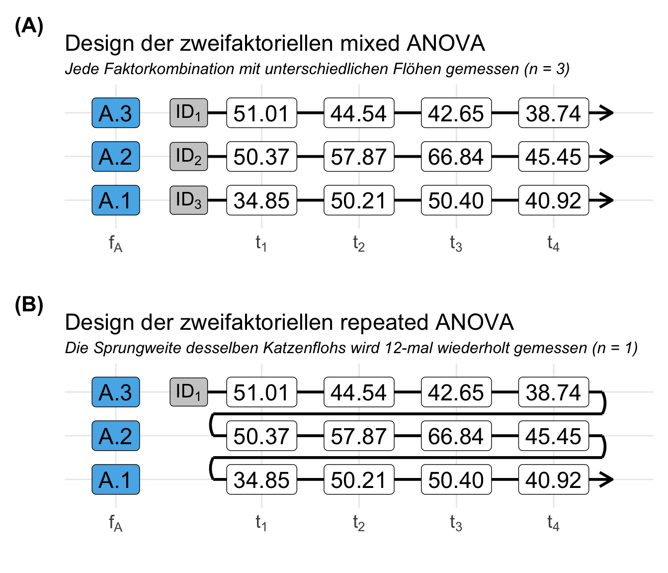
Das klingt jetzt etwas kompliziert und deshalb habe ich dir den Zusammenhang einmal in der folgenden Abbildung 34.1 visualisiert. Nehmen wir einmal an, du hast einen Behandlungsfaktor \(f_A\) mit drei Leveln. Jedes Level steht für eine Art der Behandlung. Wenn wir uns jetzt eine mixed ANOVA anschauen, dann haben wir drei Individuen vorliegen, die wiederholt in der gleichen Art der Behandlung gemessen werden. Das Individium mit der \(ID_1\) erhält nur die Behandlung \(A.3\) wiederholt verabreicht oder steht unter dieser Behandlung. Dann messen wir wiederholt den Messwert.
Etwas anders sieht es dann bei der repeated ANOVA aus. Hier haben wir ein Individum was alle Behandlungen über alle Zeitpunkte erhält. Damit erhät das Individium \(ID_1\) erst die Behandlung \(A.3\) viermal und danach dann die beiden anderen Behandlungen auch jeweils viermal wiederholt gemessen. Das ist ein großer konzeptioneller Unterschied in dem Versuchsdesign zwischen der mixed und der repeated ANOVA. In beiden ANOVA Typen wird wiederholt gemessen. In der repeated ANOVA erhält jedes Individum aber auch alle Behandlungen über die Zeit.
Bevor wir jetzt weiter in das Modell und die einzelnen Besonderheiten der mixed ANOVA und repeated ANOVA einsteigen nochmal der Hinweis, dass wir hier natürlich auch wieder nur global einen Fakor testen. Das heißt, du weißt natürlich wieder nicht, welcher paarweise Vergleich innerhalb eines Faktors einen signifikanten Unterschied ausmacht, wenn du eine signifikante ANOVA vorliegen hast. Dann musst du wieder weiter machen mit einem Post-hoc Test. Auch hier hilft nochmal die Vingette von {afex} mit ANOVA and Post-Hoc Contrasts. Oder wie es Gueorguieva & Krystal (2004) mit der wissenschaftlichen Veröffentlichung Move Over ANOVA und der Nutzung von linearen gemischten Modellen wie folgt beschreibt.
“Mixed-effects models use all available data, can properly account for correlation between repeated measurements on the same subject, have greater flexibility to model time effects, and can handle missing data more appropriately. Their flexibility makes them the preferred choice for the analysis of repeated measures data” — Gueorguieva & Krystal (2004)
Warum machen wir das nicht immer? Also wir nutzen immer ein lineares gemischtes Modell? Das hat meistens mit der geringen Anzahl an Beobachtungen in den Gruppen und allgemein mit zu wenigen Gruppen zu tun. Häufig reicht eben das Design und die Wiederholungen nicht aus für ein sauberes gemischtes Modell. Deshab ist dann eine Lösung sich die Sachlage einmal in einer mixed oder repeated ANOVA anzuschauen. Es gilt wie immer, komplexe Fragestellungen kann man meistens nicht in einem einfachen Satz beantworten. Hier kommt es dann auch wieder auf die konkrete Fragestellung an.
Welche Pakete gibt es eigentlich?
Wenn um die Anwendung der mixed oder repeated ANOVA in R geht, dann haben wir eine Menge Pakete zur Auswahl. Wie immer macht die Fragestellung und das gewählte Modell den Großteil der Entscheidungsindung aus. Ich zeige dir später in der Anwendung dann auch alle Pakete einmal, gebe dir dann aber auch immer eine Empfehlung mit. Normalerweise brauchen wir einen normalverteilten Messwert \(y\) und Varianzhomogenität in den Faktoren. In den letzten Jahren wurden aber noch weitere Implementierungen der ANOVA entwickelt, so dass hier auch Alternativen vorliegen.
Gehen wir jetzt mal die Pakete durch. Wir immer gibt es einiges an Möglichkeiten und ich zeige dir hier eben die Auswahl. Es gibt hier das ein oder andere noch zu beachten, aber da gehe ich dann bei den jeweiligen Methoden drauf ein. Es macht eben dann doch einen Unterschied ob ich eine einfaktorielle oder komplexere ANOVA rechnen will. Nicht alles geht in allen R Pakten oder gar Excel.
- Der Standard mit der Funktion
aov()aus{base} -
Die Standardfunktion
aov()erlaubt es eine mixed oder repeated ANOVA direkt auf einem Datensatz zu rechnen. Hier brauchen wir nur ein Modell in der in R üblichen Formelschreibweisey ~ f. Du kannst diesen Ansatz als schnelle ANOVA begreifen. Dein Messwert \(y\) muss hier normalverteilt sein. - Mit der Funktion
anova_test()aus{rstatix} -
Das R Paket
{rstatix}bietet bietet die Funktionanova_test()die es erlaubt einfacher auf die Funktionalität der Funktionaov()und R Funktionen aus dem Paket{car}zuzugreifen. Es ist eben ein klassischer Wrapper um besser rechnen zu können. Aber auch hier musst du verstehen wie die Funktion funktioniert. Ich finde aber die Anwendung relativ einfach und deshalb zeige ich die Funktion hier einmal. - Mit den ANOVA Funktionen aus
{afex} -
Wir können die mixed oder repeated ANOVA anwenden, wenn wir Messwiederholungen vorliegen haben. Daher bietet sich hier insbesondere das R Paket
{afex}an. Du musst bei den Funktionen von{afex}immer eine ID mitlaufen lassen, die angibt welche Individuen wiederholt gemessen wurden. Also hat jede Zeile eine Nummer, die beschreibt welche Beobachtung hier vorliegt. Besonders wichtig bei Messungen über die Zeit. Darüber hinaus kann das Paket sehr gut Interaktionen schätzen und Bedarf dort keiner zusätzlichen Optionen. Auch hier hilft nochmal die Vingette von{afex}mit ANOVA and Post-Hoc Contrasts weiter, wenn es um den Post-hoc Test geht. - Mit den ANOVA Funktionen aus
{MANOVA.RM} -
Das R Paket
{MANOVA.RM}von Friedrich et al. (2019) bietet eine weitere Möglichkeit die reapted und mixed ANOVA zu rechnen, wenn die Annahme an die Normalverteilung sowie der Varianzhomogenität nicht erfüllt ist. Wir haben es hier dann nochmal mit einer neueren Implementierung zu tun. Eine weitere robuste Alternative zu den Standardimplementierungen. - Mit den ANOVA Funktionen aus
{WRS2} -
Eine Annahme an die mixed oder repeated ANOVA ist, dass wir es mit normalverteilten Messwerten \(y\) sowie Varianzhomogenität in den Faktoren \(f\) vorliegen haben. Das R Paket
{WRS2}mit der hervorragenden Vingette Robust Statistical Methods Using WRS2 erlaubt nun aber diese beiden Annahmen zu umgehen und bietet eine robuste ANOVA an. Robust meint hier, dass wir uns nicht um die Normalverteilung und Varianzhomogenität kümmern müssen.
Wir immer ist es hier ein Tutorium um gleich mit der ANOVA starten zu können. Wenn du tiefer in die Materie einsteigen möchtest und noch andere Dinge rechts und links anschauen willst, dann findest du in den folgenden Quellen nochmal mehr Anregungen. Es geht wie immer mehr, aber wir wollen hier dann ja auch fertig werden und haben beschlossen eine repeated oder mixed ANOVA zu rechnen.
TippWeitere Tutorien für die repeated & mixed ANOVA
Wir oben schon erwähnt, kann dieses Kapitel nicht alle Themen der repeated und mixed ANOVA abarbeiten. Insbesondere der theoretische Hintergrund ist ja bei mir hier sehr gekürzt. Daher präsentiere ich hier eine Liste von Literatur und Links, die mich für dieses Kapitel hier inspiriert haben. Nicht alles habe ich genutzt, aber vielleicht ist für dich was dabei.
- Im Tutorium zur Repeated Measures ANOVA in R und Mixed ANOVA in R auf der Seite Datanovia wird nochmal mehr auf die möglichen Vortest der Annahmen eingegangen. Auch wird nochmal der Posthoc-Test gezeigt, den ich ja ausgelagert habe.
- Das Kapitel zu den Random Effects aus dem Openbook Data Analysis in R gibt nochmal einen Einblick in die Idee der zufälligen Effekte, die wir hier bewusst etwas unter den Tisch fallen lassen.
- Das Openbook ANOVA and Mixed Models A Short Introduction Using R gibt in dem Kapitel zu Random and Mixed Effects Models nochmal eine Übersicht über die verschiedenen Modelle. Insbesondere der Theorieteil ist gut, da ich ja hier in diesem Kapitel aktuell auf eine theoretische Betrachtung verzichtet habe.
- Wenn dich die Formelschreibweise in R verwirrt, dann hilft dir nochmal der Blogeintrag zu ANOVA and other models, mixed and fixed.
34.2 Genutzte R Pakete
Wir wollen folgende R Pakete in diesem Kapitel nutzen.
R Code [zeigen / verbergen]
pacman::p_load(tidyverse, magrittr, broom, WRS2, scales,
               readxl, see, car, patchwork, rstatix, emmeans,
               interactions, effectsize, afex, report, multcomp,
               janitor, MANOVA.RM, ggrepel, conflicted)
conflicts_prefer(dplyr::mutate)
conflicts_prefer(dplyr::summarize)
conflicts_prefer(dplyr::filter)
conflicts_prefer(dplyr::arrange)
conflicts_prefer(dplyr::select)
conflicts_prefer(magrittr::set_names)
conflicts_prefer(magrittr::extract)
conflicts_prefer(effectsize::eta_squared)
cbbPalette <- c("#000000", "#E69F00", "#56B4E9", "#009E73",
                "#F0E442", "#0072B2", "#D55E00", "#CC79A7")
An der Seite des Kapitels findest du den Link Quellcode anzeigen, über den du Zugang zum gesamten R-Code dieses Kapitels erhältst.
34.3 Daten
Beginnen wir wie immer mit den Daten. Hier ist die Besonderheit, dass wir immer Messweiderholungen an einer Beobachtung vorliegen haben. Ich habe dann die jeweilige Beobachtung in der Spalte .id jeweils genau benannt. Daher kommt eben die Beobachtung mit der id gleich 1 mehrfach in den Daten vor. Genauer, wir haben eben nicht nur eine Zeile in den Daten für eine Beobachtung sondern mehrere Zeilen für eine Beobachtung vorliegen. Das ist am Anfang immer etwas verwirrend, aber man gewöhnt sich daran.
Eine weitere Besonderheit ist, dass wir häufig die Daten in einem Wide-Format erstellen. Das geißt wir haben pro Zeile eine ID und dann mehrere Spalten wo wir wiederholt messen. Wir nennen dann diese Spalten meistens t0 bis t5, wenn wir sechs Zeitpunkte bemessen. In R brauchen wir dann doch wieder das Long-Format und dementsprechend nutzen wir die Funktion pivot_longer() um uns aus den Daten im Wide-Format die entsprechenden Daten im Long-Format zu bauen. Das Openbook R for Data Science hat hier noch das passende Kapitel zum nachlesen. Du kannst auch das Cheatsheet nochmal anschauen, dort wird alles nochmal visuell erklärt.
34.3.1 Mixed ANOVA
Bei der mixed ANOVA haben wir mindestens ein zweifaktorielles Design vorliegen. Warum ist das so? Zum einen brauchen wir einen Behandlungsfaktor und dazu kommt dann noch der Faktor der Messwiederholung. Wir messen ja wiederholt und dieses wiederholte Messen kommt dann ebenfalls in einen Faktor rein. Somit haben wir einen Behandlungsfaktor und einen Zeitfaktor in den Daten. Manchmal erhöhen wir noch die Komplexität und ergänzen einen zweiten Behandlungsfaktor und haben dann einen dreifaktoriellen Datensatz vorliegen.
Zweifaktoriell
Im Folgenden siehst du einmal einen Datensatz für eine zweifaktorielle mixed ANOVA. In diesem Beispiel schauen wir uns nur Katzenflöhe an. Wir haben in dem Datensatz einmal den Faktor feeding als die Fütterungsarten mit einer Kontrolle als Zuckerwasser, Blut und einmal Ketchup sowie als zweiten Faktor die verschiedenen Zeitpunkte der Messung der Sprungweite in [cm]. Wir haben an insgesamt sechs Zeitpunkten wiederholt die Sprungweite gemessen. Wir wollen nun wissen, in wie weit sich die Sprungweite über die Zeit für die drei Floharten ändert.
R Code [zeigen / verbergen]
mixed_fac2_tbl <- read_excel("data/fleas_complex_data.xlsx",
                             sheet = "mixed-fac2") |>
  select(.id, feeding, t0:t5) |>
  pivot_longer(cols = t0:t5,
               values_to = "jump_length",
               names_to = "time_fct") |>
  mutate(feeding = as_factor(feeding),
         time_fct = as_factor(time_fct),
         jump_length = round(jump_length, 2),
         .id = as_factor(.id))
In der folgenden Tabelle siehst du einmal die rohen Daten eingelesen. Wir haben den Faktor feeding sowie die sechs Zeitpunkte der Messung der Sprungweite in [cm]. Wir müssen uns dann in R die Daten über die Funktion pivot_longer() in ein Long-Format umwandeln.
| .id | feeding | t0 | t1 | t2 | t3 | t4 | t5 |
|---|---|---|---|---|---|---|---|
| 1 | ctrl | 31.56 | 27.61 | 26.12 | 17.66 | 18.33 | 7.43 |
| 2 | ctrl | 32.87 | 26.12 | 28.23 | 19.25 | 12.01 | 8.75 |
| 3 | ctrl | 33.43 | 31.23 | 26.59 | 24.19 | 13.95 | 0.27 |
| 4 | ctrl | 24.88 | 30.47 | 26.82 | 23.77 | 20.71 | 1.34 |
| ... | ... | ... | ... | ... | ... | ... | ... |
| 21 | ketchup | 48.68 | 47.28 | 33.81 | 21.89 | 27.6 | 33.84 |
| 22 | ketchup | 51.56 | 49.85 | 37.17 | 30.66 | 27.67 | 35.03 |
| 23 | ketchup | 53.51 | 47.6 | 33.31 | 30.46 | 25.32 | 28.31 |
| 24 | ketchup | 49.38 | 42.85 | 31.99 | 34.09 | 27.1 | 34.81 |
Jetzt habe ich dir in der folgenden Abbildung auch nochmal das Versuchsdesign aufgezeigt. Wie du siehst, haben wir immer einen Floh, der eine Behandlung mit einer Fütterungsart erhält. Dieser Flog springt dann zum Beispiel unter der Fütterung mit Ketchup sechs Mal und wir notieren jedesmal die Sprungweite zu den Messzeitpunkten.
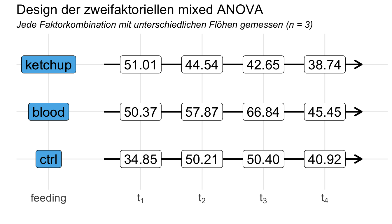
feeding. Jeder Floh erhält eine Fütterung und anschließend wird sechs mal die Sprungweite gemessen. Hier sind nur vier Zeitpunkte dargestellt. [Zum Vergrößern anklicken]
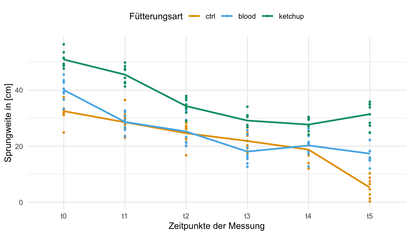
In der folgenden Abbildung siehst du dann nochmal den Zusammenhang zwischen der Sprungweite in [cm] der Katzenflöhe unter unterschiedlichen Fütterungsarten. Dabei wurden die Flöhe wiederholt an sechs Zeitpunkten gemessen. Wir du siehst, fällt mit der Zeit die Sprungleistung ab. Die Katzenflöhe springen unabhängig von der Fütterungsart weniger weit mit der Zeit. Am letzten Zeitpunkt scheinen die Flöhe unter Ketchupernährung dann wieder etwas weiter zu springen. Jetzt müssen wir aber einmal statistisch Nachweisen, ob wir hier wirklich einen signifikanten Zusammenhang und Unterschiede zwischen den Fütterungsarten vorliegen haben.
Dreifaktoriell
Für unser dreifaktorielles Beispiel erweiter wir einmal den Datensatz um ein Workout für die Katzenflöhe. Neben den drei Fütterungsarten Kontrolle mit Zuckerwasser, Blut sowie Ketchup mussten die Flöhe als zweiten Faktor noch ein Workout bestehen. Dabei haben nicht alle Katzenflöhe jeweils trainiert, sondern wir haben eine untrainierte Gruppe sowie eine trainierte Gruppe. Beide Gruppen des Workout wurden dann mit allen drei Fütterungsarten gefüttert. Dann wurden insgesamt zu sechs Zeitpunkten die Sprungweite in [cm] bestimmt. Wir haben es daher mit einem dreifaktoriellen Datensatz zu tun, da wir zwei Behandlungsfaktoren sowie den Faktor der Messwiederholungen in unseren Daten vorliegen haben.
R Code [zeigen / verbergen]
mixed_fac3_tbl <- read_excel("data/fleas_complex_data.xlsx",
                             sheet = "mixed-fac3") |>
  select(.id, feeding, workout, t0:t5) |>
  pivot_longer(cols = t0:t5,
               values_to = "jump_length",
               names_to = "time_fct") |>
  mutate(feeding = as_factor(feeding),
         workout = as_factor(workout),
         time_fct = as_factor(time_fct),
         jump_length = round(jump_length, 2),
         .id = as_factor(.id))
In der folgenden Tabelle sind die Daten dann nochmal im Wide-Format dargestellt. Wir haben hier dann pro Floh jeweils eine Faktorkombination aus der Fütterungsart feeding sowie dem Traingsstatus workout. Im Anschluss haben wir dann die Sprungweite von jedem Floh sechsmal gemessen. Wir müssen dann in R die Daten nochmal in das Long-Format über die Funktion pivot_longer() umbauen.
| .id | feeding | workout | t0 | t1 | t2 | t3 | t4 | t5 |
|---|---|---|---|---|---|---|---|---|
| 1 | ctrl | yes | 44.5 | 32.4 | 33.02 | 18.14 | 20.88 | 10.78 |
| 2 | ctrl | yes | 36.33 | 37.05 | 31.79 | 25.72 | 28.01 | 8.79 |
| 3 | ctrl | yes | 31.76 | 31.75 | 29.82 | 26.39 | 27.4 | 15.52 |
| 4 | ctrl | yes | 38.28 | 37.08 | 30.53 | 27.8 | 28.37 | 5.21 |
| ... | ... | ... | ... | ... | ... | ... | ... | ... |
| 21 | ketchup | no | 59.12 | 51.66 | 35.64 | 39.56 | 27.77 | 32.88 |
| 22 | ketchup | no | 53.51 | 58.28 | 36.65 | 34.62 | 28.09 | 38.01 |
| 23 | ketchup | no | 62.22 | 48.53 | 46.73 | 34.81 | 34.2 | 29.03 |
| 24 | ketchup | no | 53.4 | 52 | 37.78 | 47.77 | 35.5 | 27.63 |
Manchmal ist es schwer die Zusammenhänge dann in dem Datensatz zu sehen, deshalb hier nochmal das Versuchsdesign visualisert. Jeder Katznfloh springt wiederholt, aber das ganz dann nur unter einer Faktorkombination.
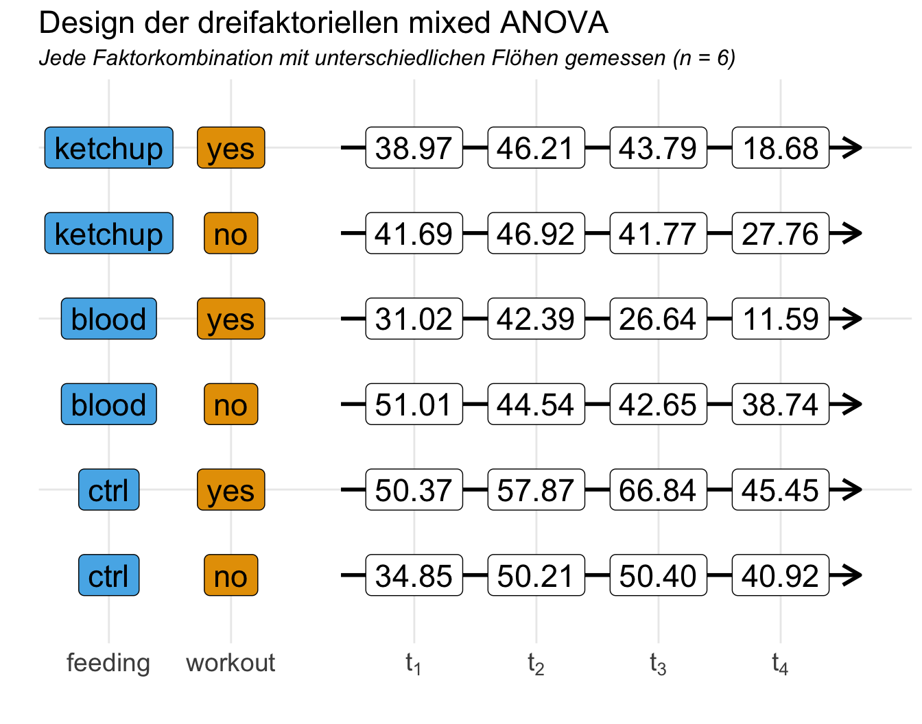
feeding. Der zweite Faktor der Status des Workouts für jeden Floh workout. Jeder Floh erhält eine Fütterung sowie ein Workout und anschließend wird sechs mal die Sprungweite gemessen. Hier sind nur vier Zeitpunkte dargestellt. [Zum Vergrößern anklicken]
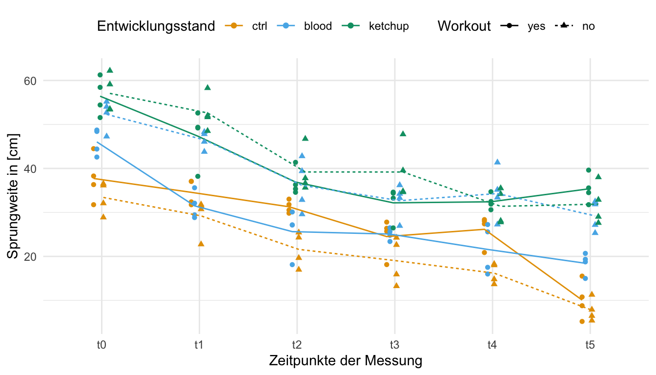
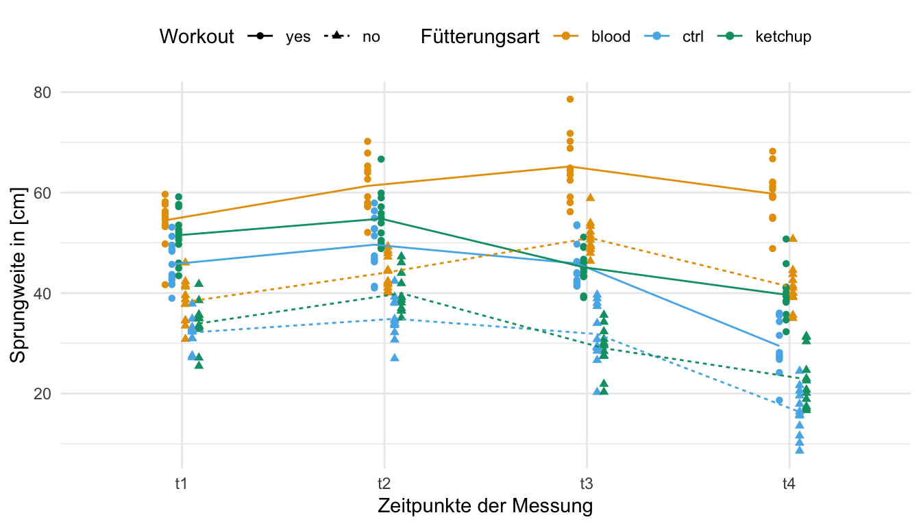
Abschließend können wir uns dann nochmal die Daten in der folgenden Abbildung anschauen. Auf den ersten Blick sehen wir, dass die Leistung in der Sprungweite über die Zeit abfällt. Diesen Trend können wir über alle Fütterungsarten beobachten. Was erst auf den zweiten Blick auffällt ist, dass teilweise ja nach Fütterungsart ein Training positiv oder negativ ausfällt. So führt ein Training bei den Kontrollflöhen zu weiteren Sprüngen. Die Katzenflöhe unter einer Blutdiät springen jedoch unter Training nicht so weit wie ohne ein Training.
34.3.2 Repeated ANOVA
Die repeated ANOVA ist in den Agrarwissenschaften selten. In den Sozialwissenschaften oder aber allgemeiner den Humanwissenschaften kommt die repeated ANOVA häufiger vor. Das hat vor allem damit zu tun, dass wir jedes Individuum mit allen Faktorkombinationen behandeln und wiederholt messen. Das wir ein Subjekt wiederholt messen kommt auch häufiger in den Agrarwissenschaften vor, aber selten erhält jedes Tier oder Pflanze alle Behandlungen verabreicht. Deshalb hier einmal die Daten für die repated ANOVA als Veranschaulichung was du als Daten und Experiment vorliegen haben musst.
Einfaktoriell
Im Gegensatz zu mxied ANOVA können wir in der repeated ANOVA auch nur den einfaktoriellen Fall vorliegen haben. Da klingt jetzt erstmal etwas seltsam, aber wir haben in diesem Fall nur die Zeitpunkte als Faktor vorliegen. Wir messen also nur Katzenflöhe ohne eine Behandlung viermal. Wir schauen also, ob sich die Sprungweite von Katzenflöhen über die Zeitpunkte verändert. Wir vergleichen faktisch also nur die Zeitpunkte untereinander.
R Code [zeigen / verbergen]
repeated_fac1_tbl <- read_excel("data/fleas_complex_data.xlsx",
                                sheet = "repeated-fac1") |>
  select(.id, animal, t1:t4) |>
  pivot_longer(cols = t1:t4,
               values_to = "jump_length",
               names_to = "time_fct") |>
  mutate(animal = as_factor(animal),
         time_fct = as_factor(time_fct),
         jump_length = round(jump_length, 2),
         .id = as_factor(.id))
Auch hier einmal die Daten im Wide-Format, damit die Daten etwas übersichtlicher sind. Wir haben nur die Katzenflöhe vorligen und schauen uns zwölf einzelne Katzenflöhe an. Jeder Floh springt dann vier Mal und wir messen dann die Sprungweite in [cm]. Wir müssen uns dann noch das Long-Format über die Funktion pivot_longer() in R bauen.
| .id | animal | t1 | t2 | t3 | t4 |
|---|---|---|---|---|---|
| 1 | cat | 23.72 | 37.57 | 36.67 | 25.89 |
| 2 | cat | 17.84 | 29.36 | 22.63 | 15.44 |
| 3 | cat | 24.11 | 30.43 | 30 | 28.14 |
| ... | ... | ... | ... | ... | ... |
| 10 | cat | 28.52 | 32.39 | 33.35 | 23.91 |
| 11 | cat | 25.46 | 29.02 | 22.68 | 19.88 |
| 12 | cat | 20.92 | 34.39 | 26.81 | 24.76 |
So ergibt sich dann auch ein sehr simples Versuchsdesign. Wir lassen jeden Katzenfloh viermal springen und messen jeweils die Sprungweite für jeden Floh.
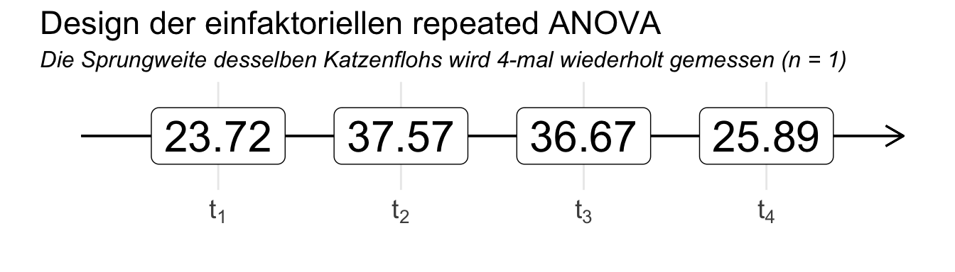
Damit ergibt sich am Ende auch eine sehr übersichtliche Abbildung. Wir sehen einmal die einzelnen Katzenflöhe. Jede Sprungweite über die vier Zeitpunkte habe ich für die individuellen Flöhe mit einer gestrichelten Linie verbunden. Den globalen Trend kannst du in der farbigen Linie nachvollziehen. Am Anfang springen die Flöhe nicht soweit, steigern sich dann zum zweiten Messzeitpunkt um dann wieder stetig abzunehmen. Einzelne Flöhe zeigen dabei eine größere Variabilität als der globale Trend.

Zweifaktoriell
Eigentlich wird die Besonderheit des repeated Design einer ANOVA erst bei der zweifaktoriellen repeated ANOVA so richtig ersichtlich. Hier haben wir es nämlich zum einen mit einem Behandlungsfaktor zu tun und einer Faktor mit den jeweiligen Messzeitpunkten. Wir haben hier wieder die Katzenflöhe mit unterschiedlichen Fütterungsarten ernährt und dann an vier Zeitpunkten gemessen, wie weit die Flöhe springen. Die Besonderheit ist jetzt, dass jeder Katzenfloh alle Behandlungen durchläuft. Das macht einen gewaltigen Unterschied im Design und in der Auswertung.
R Code [zeigen / verbergen]
repeated_fac2_tbl <- read_excel("data/fleas_complex_data.xlsx",
                                sheet = "repeated-fac2") |>
  select(.id, animal, feeding, t1:t4) |>
  pivot_longer(cols = t1:t4,
               values_to = "jump_length",
               names_to = "time_fct") |>
  mutate(animal = as_factor(animal),
         feeding = as_factor(feeding),
         time_fct = as_factor(time_fct),
         jump_length = round(jump_length, 2),
         .id = as_factor(.id))
In der folgenden Tabelle der Rohdaten der Sprungweiten in [cm] unserer Katzenflöhe siehst du nochmal die Besonderheit der Messwiederholung. Wir messen die Sprungweite von jedem Floh \(.id\) viermal für jede Fütterungsart. Wir müssen natürlich zwischen den Fütterungsarten Zeit lassen, damit wir wieder die Fütterungseffekte raus haben, aber ansonsten wird jeder Floh mit allen Ernährungsformen gefüttert. Hier ist dann auch die \(.id\) Spalte so wichtig, da wir ja wissen müssen welche Fütterungsart zu welchem Floh gehört. Abschließend nutzen wir die Funktion pivot_longer() um uns die Daten passend in R zusammenzubauen.
| .id | animal | feeding | t1 | t2 | t3 | t4 |
|---|---|---|---|---|---|---|
| 1 | cat | ctrl | 34.85 | 50.21 | 50.4 | 40.92 |
| 1 | cat | blood | 50.37 | 57.87 | 66.84 | 45.45 |
| 1 | cat | ketchup | 51.01 | 44.54 | 42.65 | 38.74 |
| 2 | cat | ctrl | 34.24 | 43.85 | 37.34 | 30.92 |
| ... | ... | ... | ... | ... | ... | ... |
| 11 | cat | ketchup | 42.29 | 49.83 | 46.08 | 39.97 |
| 12 | cat | ctrl | 42.88 | 46.23 | 45.93 | 29.81 |
| 12 | cat | blood | 49.9 | 56.72 | 66.54 | 47.85 |
| 12 | cat | ketchup | 46.47 | 52.61 | 44.92 | 33.58 |
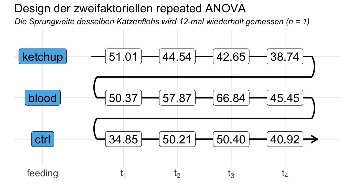
In der folgenden Abbildung siehst du dann das Versuchsdesign für einen Katzenfloh nochmal dargestellt. Der Floh beginnt mit der Ernährungsform ketchup und springt dann viermal. Jedes Mal messen wir dann die Sprungweite. Nach einer Pause erhält der gleiche Katzenfloh dann die Ernährungsform blood und springt wieder zeitversetzt viermal. Am Ende ernähren wir dann den Floh noch mit Zuckerwasser ctrl und lassen ihn abschließend viermal springen. Damit springt ein einzelner Katzenfloh über den Versuch hinweg zwölfmal unter verschiedenen Versuchsbedingungen. Wie du siehst, ist dieses Design vermutlich nicht so häufig in den Agrarwissenschaften anzutreffen.
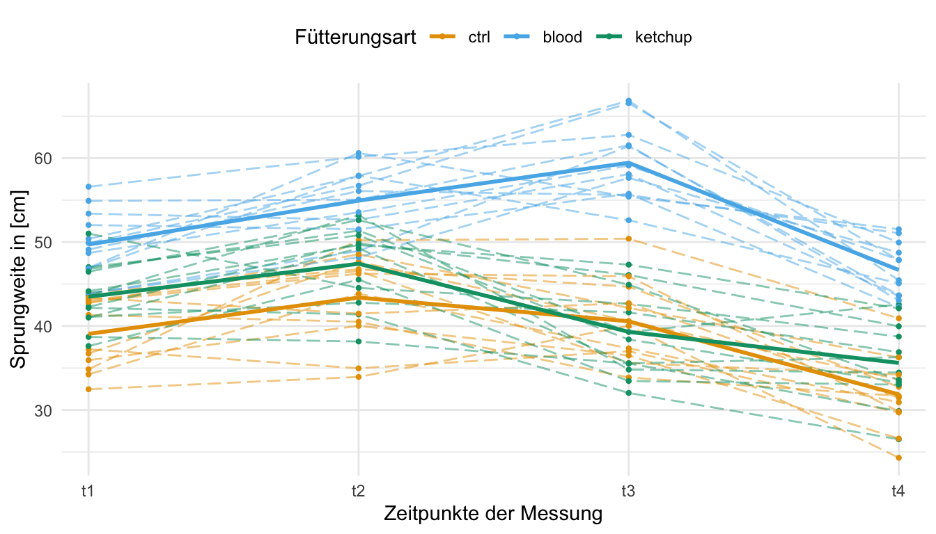
Dann schauen wir uns nochmal den Zusammenhang zwischen der Ernährungsart und den einzelnen Zeitpunkten einmal in einer Abbildung an. Die einzelnen Flöhe sind als getrichelte Linien dargestellt. Die durchgezogenen Linien stellen die globalen Mittelwerte an den jeweiligen Zeitpunkten für die Fütterungsart dar. Wir sehen, dass wir Unterschiede in den Sprungweiten über die Zeitpunkte je nach Ernährungsform vorliegen haben. Dabei haben die Kontrolle und der Ketchup ähnliche Verläufe.
Dreifaktoriell
Jetzt wird es richtig wild. Wir schauen uns jetzt nämlich nicht nur einen Behandlungsfaktor an, sondern haben zwei Behandlungen sowie die Messwiederholungen als Faktor über die Zeit. Wir schauen hier einmal auf die Fütterungsart mit der Kontrolle als Zuckerwasser, der Gabe von Blut sowie der Fütterung mit Ketchup. Dazu kommt dann noch eine Workoutsession oder eben keine Workoutsession. Wir haben damit zwei Behandlungsfaktoren vorliegen. Da wir ja nun jeden Floh wiederholt messen unter jeder Faktorkombination, kommt hier einiges an Sprungweitenmessung auf jeden einzelnen Floh zu. Daher sind repeated ANOVAs selten. Wir müssen ja nicht nur jeden Floh wiederholt für die Fütterungen durchmessen sondern eben auch nochnmal alles wiederholt für die beiden Workoutgruppen.
R Code [zeigen / verbergen]
repeated_fac3_tbl <- read_excel("data/fleas_complex_data.xlsx",
sheet = "repeated-fac3") |>
select(.id, animal, feeding, workout, t1:t4) |>
pivot_longer(cols = t1:t4,
values_to = "jump_length",
names_to = "time_fct") |>
mutate(animal = as_factor(animal),
feeding = as_factor(feeding),
workout = as_factor(workout),
time_fct = as_factor(time_fct),
jump_length = round(jump_length, 2),
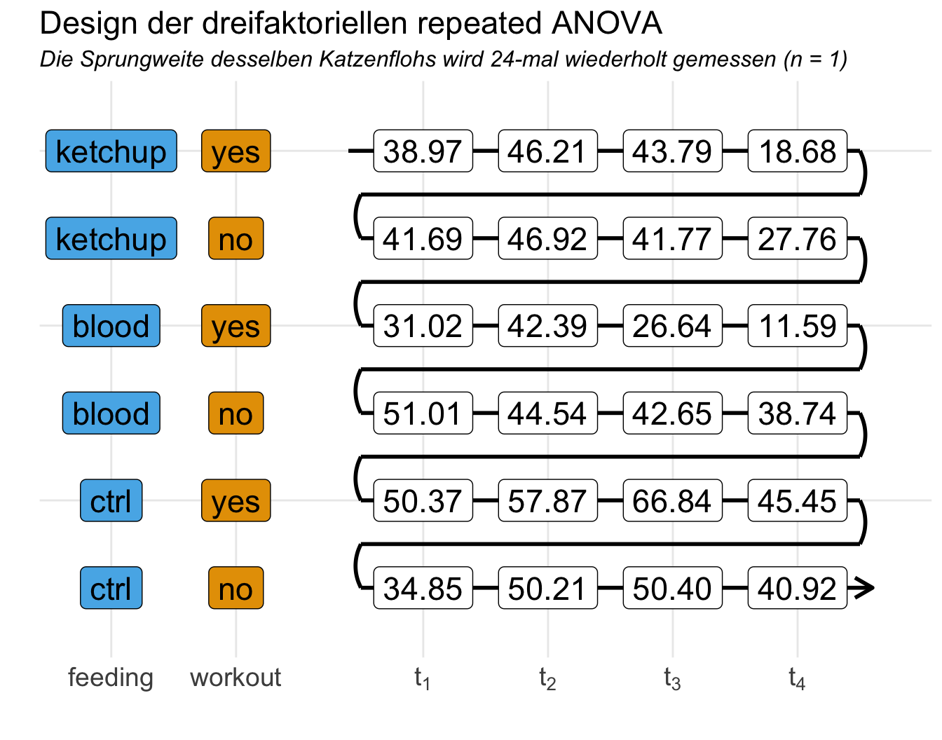
.id = as_factor(.id))In der folgenden Tabelle siehst du einmal die Daten im Wide-Format. In den ersten beiden Zeilen siehst du auch schon die Besonderheit. Wir Füttern eben einmal mit Bkut und messen dann viermal die Sprungweite für die beiden Gruppen des Workout. Daher messen wir dann jeden Floh insgesamt vierundzwanzigmal mit den jeweiligen Pausen zwischen den Behandlungskombinationen. Da kommen schon eine Menge Sprünge zusammen.
| .id | animal | feeding | workout | t1 | t2 | t3 | t4 |
|---|---|---|---|---|---|---|---|
| 1 | cat | blood | yes | 57.62 | 67.87 | 68.82 | 61.19 |
| 1 | cat | blood | no | 42.32 | 49.28 | 58.87 | 50.75 |
| 1 | cat | ctrl | yes | 49.53 | 54.91 | 46.01 | 34.32 |
| 1 | cat | ctrl | no | 31.02 | 42.39 | 26.64 | 11.59 |
| ... | ... | ... | ... | ... | ... | ... | ... |
| 12 | cat | ctrl | yes | 48.82 | 52.84 | 41.37 | 36.02 |
| 12 | cat | ctrl | no | 32.85 | 32.18 | 29.1 | 16.41 |
| 12 | cat | ketchup | yes | 59.16 | 55.02 | 39.41 | 41.03 |
| 12 | cat | ketchup | no | 35.11 | 36.99 | 27.43 | 30.36 |
Eigentlich sieht man das Versuchsdesign erst so richtig in der folgenden Abbildung. Hier siehst du einmal wie ein einzelner Floh alle 24 Sprünge nacheinander unter der jeweiligen Faktorkombination durchführt. In einem idealen Setting folgt natürlich jeder Floh eine zufällige Reihenfolge der Faktorkombinationen. Bitte beachte, dass zwischen den einzelnen Behandlungskombinationen nach dem vierten Sprung natürlich auch eine Zeit vergehen muss, damit sich die Behandlung wieder ausgeschlichen hat.
Am Ende schauen wir uns auch die Daten einmal in einer Abbildung an. Hier haben wir dann die beiden Workoutgruppen sowie die drei Fütterungsarten in einer Abbildung vereint. Wir sehen, dass die nicht trainierten Flöhe im allgemeinen nicht so weit springen wir die trainierten Flöhe. Ebenso wirkt, dass die Ernährung mit Blut auf jeden Fall die bessere Sprungleistung bewirkt. Teilweise sehen wir, dass sich die Linien der Mittelwerte überschneiden, so dass wir hier eventuell von einer Interaktion ausgehen müssen. Das schauen wir uns dann aber in den entsprechenden statistischen Tests einmal näher an.
34.4 Mixed ANOVA
Beginnen wir mit der Auswertung unserer beispieldaten mit der mixed ANOVA. Wir kriegen hier natürlich nur eine globale Aussage über den Faktor der Behandlung oder der Zeit. Wenn dich die paarweisen Vergleiche interessieren, dann müsst du noch einen Posthoc-Test anschließen. Mehr Informationen zu der Modellierung findest du auch in dem Kapitel zu gemischten Modellen. Dort erfährst du dann auch, wie du dir den Posthoc-Test bauen kannst. Hier bleiben wir dann bei der ANOVA und den entsprechenden Ergebnissen.
34.4.1 Zweifaktoriell
Als erstes schauen wir uns die Auswertung der zweifaktoriellen mixed ANOVA an. Nochmal zur Erinnerung, wir haben einen Behandlungsfaktor mit den drei Arten der Fütterung, Kontrolle, Blut und Ketchup, vorliegen. Darüber hinaus messen wir die Sprungweite an sechs Zeitpunkten widerholt für jeden Katzenfloh. Wir wollen jetzt wissen, ob die Fütterung einen Einfluss auf die Sprungweiten der Katzenflöhe über die Zeit hat. Dabei sind wir eigentlich nicht so sehr an den Zeitpunkten wie an der Behandlung der Fütterung interessiert. In einem zweifaktoriellen Versuch können wir uns dann auch immer die Interaktion mit anschauen um zu sehen, die Behandlung unabhängig von den Zeitpunkten ist.
Die Standardimplementierung ist eigentlich recht einfahc durchzuführen. Wir haben wie immer erst unseren Messwert \(y\) und dann die Formelschreibweise für unser beiden Faktoren und deren Interaktion. Ich mache mir es hier etwas einfacher und schreibe dann noch die Faktoren mit dem * um etwas Platz zu sparen. Die Besonderheit hier ist jetzt, dass wir noch spezifizieren müssen welche Variable in unseren Daten die wiederholt gemessenen Individuen darstellt und über welchen Faktor diese Individuen dann wiederholt gemessen wurden. In unserem Fall stehen die Individuen in der Spalte .id und wir haben über die Spalte time_fct wiederholt die einzelnen Flöhe gemessen. Dann müssen wir das ganze noch in die Funktion Error() schreiben, damit die ANOVA auch erkennt, dass wir hier den Teil mit den Messwiederholungen darstellen.
R Code [zeigen / verbergen]
aov(jump_length ~ feeding * time_fct + Error(.id/time_fct),
    data = mixed_fac2_tbl) |>
  tidy() |>
  na.omit() |>
  select(term, df, statistic, p.value) |>
  mutate(p.value = pvalue(p.value))
# A tibble: 3 × 4
term df statistic p.value
<chr> <dbl> <dbl> <chr>
1 feeding 2 214. <0.001
2 time_fct 5 116. <0.001
3 feeding:time_fct 10 8.49 <0.001 Ich filtere hier einiges weg, da wir hier viele Informationen erhalten, die wir meistens nicht brauchen. Wir sehen, dass einen signifikanten Einfluss der Fütterung auf die Sprungweite haben, da der p-Wert kleiner ist als das Signifikanzniveau \(\alpha\) gleich 5%. Dies ist auch der Fall für die Zeitpunkte und die Interaktion. Da wir hier eine signifikante Interaktion vorliegen haben, können wir die Fütterungsarten nicht unabhängig über die Zeit interpretieren. Es gibt damit Zeitpunkte an denen die Fütterungen unterschiedliche Effekte zeigen.
Das R Paket {rstatix} liefert mit der Funktion anova_test() auch eine Möglichkeit eine mixed ANOVA zu rechnen. Hier ist es dann mit den Optionen etwas anders. Ich mag ja die Formelschreibweise sehr gerne, da weiß ich dann wo was steht. Auf der anderen Seite mag es aber auch einfacher sein, wenn man einfach die Variablen in den Daten einer Option in der Funktion zuordnet. Hier haben wir den Fall, dass wir sagen müssen, was ist unser Messwert? Der Messwert kommt in die Option dv. Dann brauchen wir die individuellen IDs in der Option wid. Die Faktoren, die wir untereinander vergleichen wollen, kommen dann in die Option between. In unserem Fall sind das die Fütterungsarten. Wir wollen wissen ob es zwischen den Fütterungsarten einen Unterschied gibt. Die Zeit als Messwiederholung kommt dann in die Option within. Wir messen ja die Zeitpunkte innerhalb (eng. within) der Individuen.
R Code [zeigen / verbergen]
rstatix_aov <- anova_test(data = mixed_fac2_tbl,
                          dv = jump_length, wid = .id,
                          between = feeding, within = time_fct)
get_anova_table(rstatix_aov)
ANOVA Table (type II tests)
Effect DFn DFd F p p<.05 ges
1 feeding 2 21 214.133 1.08e-14 * 0.750
2 time_fct 5 105 115.543 4.79e-41 * 0.824
3 feeding:time_fct 10 105 8.488 5.19e-10 * 0.408Numerisch sind die Werte die gleichen Werte, die wir auch in der aov() Funktion erhalten. Im Hintergrund wird auch eine aov() gerechnet, nur die Übergabe der Variablen ist hier anders. Neben der Signifikanz kriegen wir in der Spalte ges auch noch ein Eta\(^2\) Wert wiedergegeben, den wir klassisch interpretieren können. Da wir es in einer mixed ANOVA mit einem etwas anderen Eta\(^2\) Wert zu tun haben, können wir hier erstmal sagen, dass je gößer der Wert desto stärker der Effekt. Die p-Werte sind auch hier für alle Vergleiche hoch signifikant.
Das R Paket {afex} elraubt im besonderen die Modellierung von Messwiederholungen von Beobachtungen. Faktisch ist das Paket um diese Art der Analyse gebaut. Dementsprechend gibt es auch zwei Arten des Funktionsaufrufs. Wir konzentrieren uns hier aus Gründen der konsistents zu aov() auf die Funktion aov_car(). Am Ende kommen hier die gleichen Werte raus wie schon bei den anderen Tabs. Wir haben hier aber die Möglichkeit etwas mehr zu machen. Alles Weitere dann in der Vingette zu {afex} und dem Posthoc-Test. Wenn du viel mit Messwiederholungen arbeitest, dann ist eine Einarbeitung in {afex} sicherlich sinnvoll. Leider bist du bei {afex} an die Normalverteilung und die Varianzhomogenität gebunden. MAn kann eben nicht alles haben.
R Code [zeigen / verbergen]
aov_car(jump_length ~ feeding * time_fct + Error(.id/time_fct),
        data = mixed_fac2_tbl)
Anova Table (Type 3 tests)
Response: jump_length
Effect df MSE F ges p.value
1 feeding 2, 21 13.29 214.13 *** .750 <.001
2 time_fct 4.11, 86.33 18.70 115.54 *** .824 <.001
3 feeding:time_fct 8.22, 86.33 18.70 8.49 *** .408 <.001
---
Signif. codes: 0 '***' 0.001 '**' 0.01 '*' 0.05 '+' 0.1 ' ' 1
Sphericity correction method: GG Auch hier erhalten wir die gleichen numwerischen Werte wie schon in den vorherigen Tabs zu {base} und {rstatix}. Die Signifikanz ist für alle Faktoren sowie der Interaktion gegeben. Wir erhalten auch hier in der Spalte ges dann das Eta\(^2\) als Effektschätzer zurück. Am Ende finde ich die Ausgabe etwas sperrig.
Das R Paket {afex} erlaubt es auch die Modelle nach der Schreibweise der linearen gemischten Modelle zu definieren. Das ist für mich eigentlich etwas angenehmer, da man sich dann in einer Formelwelt aufhält mehr dazu dann im Kapitel zu gemischten Modellen. Also die Ergebnisse sind die Gleichen. Ich brauche es nur als Referenz für mich zum nachschlagen.
R Code [zeigen / verbergen]
aov_4(jump_length ~ feeding * time_fct + (time_fct|.id),
      data = mixed_fac2_tbl)
Mit dem R Paket {MANOVA.RM} haben wir auch die Möglichkeit eine mixed ANOVA zu rechnen in dem wir die Funktion RM() nutzen. Das ist natürlich etwas verwirrend vom Namen, aber wenn wir die Optionen richtig mit den Variablen belegen, dann rechnen wir auch eine mixed ANOVA. Hier müssen wir dann angeben in welche Spalte die Beobachtungen sind und was der within Faktor ist. Bei uns ist das dann einfach. Wir nutzen die Variable .id sowie als Faktor der Messwiederholungen time_fct. Der Rest ist eigentlich nicht so wichtig. Wenn du die Funktion in deiner Analyse rechnest, dann würde ich die Option iter auf 1000 setzen.
Am Ende muss sich aber dann doch fragen, ob es eine noch hässlichere Ausgabe einer Funktion gibt. Ich glaube eher nicht, aber das soll die Leistung des Algorithmus nicht schmälern. Wir kämpfen uns da doch mal durch. Manche Informationen sind dann einfach auch wieder über, da wir je eigentlich nur wissen wollen, ob wir einen signifikanten Einfluss der Behandlung feeding vorliegen haben.
R Code [zeigen / verbergen]
RM(jump_length ~ feeding * time_fct, data = mixed_fac2_tbl,
   subject = ".id", within = c("time_fct"), iter = 100,
   resampling = "Perm", seed = 1234) |>
  summary()
Call:
jump_length ~ feeding * time_fct
A repeated measures analysis with 1 within-subject factor(s) ( time_fct ) and 1 between-subject factor(s).
Descriptive:
feeding time_fct n Means Lower 95 % CI Upper 95 % CI
1 ctrl t0 8 32.510 27.041 37.979
4 ctrl t1 8 28.544 22.315 34.773
7 ctrl t2 8 24.625 19.272 29.978
10 ctrl t3 8 21.853 17.032 26.673
13 ctrl t4 8 18.774 12.618 24.929
16 ctrl t5 8 5.239 0.156 10.321
2 blood t0 8 40.072 34.510 45.635
5 blood t1 8 28.651 24.154 33.148
8 blood t2 8 25.236 17.146 33.327
11 blood t3 8 18.062 11.397 24.728
14 blood t4 8 20.250 14.413 26.087
17 blood t5 8 17.351 11.442 23.260
3 ketchup t0 8 50.941 46.864 55.018
6 ketchup t1 8 45.538 41.039 50.036
9 ketchup t2 8 34.306 30.118 38.494
12 ketchup t3 8 29.146 23.946 34.346
15 ketchup t4 8 27.706 24.583 30.830
18 ketchup t5 8 31.434 25.615 37.252
Wald-Type Statistic (WTS):
Test statistic df p-value
feeding "396.501" "2" "<0.001"
time_fct "1009.823" "5" "<0.001"
feeding:time_fct "83.636" "10" "<0.001"
ANOVA-Type Statistic (ATS):
Test statistic df1 df2 p-value
feeding "214.133" "1.982" "72.609" "<0.001"
time_fct "115.543" "4.111" "Inf" "<0.001"
feeding:time_fct "8.488" "6.975" "Inf" "<0.001"
p-values resampling:
Perm (WTS)
feeding "<0.001"
time_fct "<0.001"
feeding:time_fct "0.02" Als erstes erhalten wir eine lange Tabelle mit der deskriptiven Statistik der Mittelwerte für jede Faktorkombination der Fütterungsart sowie dem Zeitpunkt. Dazu dann noch die passenden 95% Konfidenzintervalle. Dann kommen drei Tests nacheinander. Das ist auch immer das Problem, wenn du dann drei Ausgaben hast und nicht weißt, welche du nehmen sollst. Ich würde hier die Ergebnisse der ANOVA-Type Statistic (ATS) nehmen und den Rest liegen lassen. Die p-Werte aus dem Permutationstest p-values resampling haben zwar auch ihre Berechtigung bei nicht normalverteilten oder varianzheterogenen Daten aber ich würde dann hier auch eher das R Paket {WRS2} vorziehen.
Kommen wir nun zum letzten Paket, was ich hier noch für die zweifaktorielle mixed ANOVA zeigen möchte. Es handelt sich um {WRS2}, welches dann auch erlaubt die zweifaktorielle mixed ANOVA zu rechnen, wenn wir die Annahme der Normalverteilung an den Messwert oder keine Varianzhomogenität in den Gruppen vorliegen haben. Es geht dann auch beides. Das ist dann auch der große Vorteil von {WRS2}. Das Modell sieht genauso aus wie auch bei den anderen Anwendungen. Wir müssen hier nur einmal in der Option id angeben, welche Spalte unsere ID ist.
R Code [zeigen / verbergen]
bwtrim(jump_length ~ feeding * time_fct, id = .id, data = mixed_fac2_tbl)Call:
bwtrim(formula = jump_length ~ feeding * time_fct, id = .id,
data = mixed_fac2_tbl)
value df1 df2 p.value
feeding 186.6213 2 9.6997 0.0000
time_fct 142.2153 5 9.7570 0.0000
feeding:time_fct 4.6665 10 9.4221 0.0133Die Ergebnisse sind dann vom p-Wert inhaltlich gleich wie bei den anderen Anwendungen. Das habe ich hier auch erwartet, denn unsere Sprungweiten habe ich so gebaut, dass die Sprungweiten normalverteilt sind. Nicht immer können wir aber in unseren Daten davon ausgehen, dass wir normalverteilte Messwerte vorliegen haben. Da ist diese Alternative hier sehr gut.
Wir haben ja in den obigen Anwendungen der mixed ANOVA immer eine signifikante Interaktion gefunden. Daher wollen wir uns einmal in einem Liniendiagramm der Mittelwerte die Sachlage näher anschauen. Wenn wir eine Interaktion erwarten, dann sollten sich die Linien der Mittelwerte kreuzen. Wir haben ja auch in allen Analysen eine signifkante Interaktion voriegen. Wenn wir jetzt auf die Abbildung schauen, dann sehen wir auch, dass sich die Lienien für die Fütterung mit Blut und der Kontrolle kreuzen. Wir haben hier eine Interaktion vorliegen. Auch sind die Unterschiede zwischend den Fütterungen nicht immer parallel zueinander mit dem gleichen Effekt oder eben Abstand.
R Code [zeigen / verbergen]
mixed_fac2_tbl |>
  ggplot(aes(x = time_fct, y = jump_length,
             color = feeding, group = feeding)) +
  theme_minimal() +
  stat_summary(fun = "mean", geom = "point") +
  stat_summary(fun = "mean", geom = "line") +
  theme(legend.position = "top") +
  scale_color_okabeito()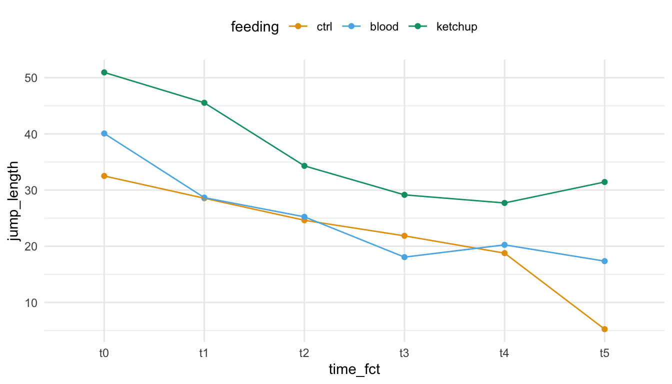
feeding und time_fct. Die Linien kreuzen sich leicht, es liegt eine Interaktion vor. Eine allgemeine Aussage über die Sprungweite und der Fütterung lässt sich nicht unabhängig vom Zeitpunkt treffen. Die Interaktion ist aber nicht sehr stark.
34.4.2 Dreifaktoriell
Jetzt betrachten wir noch die dreifaktorielle mixed ANOVA. Dieses Design kommt dann vor, wenn du zwei Behandlungsfaktoren sowie einen Zeitfaktor in deinen Daten vorliegen hast. In unserem Fall ist der erste Faktor die Fütterungsart mit den Gruppen Kontrolle, Blut und Ketchup sowie als zweiten Faktor der Status des Workouts des einzlenen Flohs. Wir schauen hier nur Katzenflöhe an. Dann messen wir die Sprungweite jedes einzelnen Flohs nochmal zu sechs Zeitpunkten. Hier ist es wieder wichtig darauf zu achten, was mit einem einzelnen Floh passiert und gemessen wird. Wir messen hier jede Faktorkombination und Wiederholung mit einem neuen Floh. Schaue dir dazu nochmal die Übersicht des Designs in dem Abschnitt zu den Daten in der Abbildung 34.4 an. Auch hier ist es dann manchmal von Vorteil zu wissen, wechler Faktor einem eigentlich am meisten interessiert. Wir betrachten hier jetzt alle drei Faktoren und deren Interaktionen als gleichwertig. Wir können die dreifaktorielle mixed ANOVA nicht mehr in dem R Paket {WRS2} rechnen. Das Paket biette keine Funktion dafür an.
Beginnen wir wieder mit der Standardfunktion in {base} mit aov() und deren Anwendung. Hier kommt dann die verkürzende Formelschreibweise mit dem Stern * zum Einsatz. Ich kann mir nicht merken was alle Faktorkombinationen zusammen mit allen Interaktionen sind. Daher nutze ich dann einmal die Schreibweise, die mir diese Überlegung abnimmt. Dann muss ich noch in dem Fehlerterm mitteilen wer .id in welchen Faktor time_fct wiederholt wird. Damit ist die dreifaktorielle mixed ANOVA der zweifaktoriellen mixed ANOVA sehr ähnlich. Wir erhalten dann folgende Ausagen, die ich nochmal aufgereinigt habe, da ich nicht alle Spalten und Informationen brauche. Auch mag ich den p-Wert gerne etwas übersichtlicher.
R Code [zeigen / verbergen]
aov(jump_length ~ feeding * workout * time_fct + Error(.id/time_fct),
    data = mixed_fac3_tbl) |>
  tidy() |>
  na.omit() |>
  select(term, df, statistic, p.value) |>
  mutate(p.value = pvalue(p.value))
# A tibble: 7 × 4
term df statistic p.value
<chr> <dbl> <dbl> <chr>
1 feeding 2 318. <0.001
2 workout 1 14.0 0.002
3 feeding:workout 2 79.0 <0.001
4 time_fct 5 113. <0.001
5 feeding:time_fct 10 4.03 <0.001
6 workout:time_fct 5 0.943 0.457
7 feeding:workout:time_fct 10 1.45 0.171 Wir sehen sofort, dass die beiden Faktoren der Fütterungsart sowie des Workout signifikant sind. Auch haben wir eine signifikante Interaktion zwischen den beiden Faktoren vorliegen. Die Gruppen der Fütterung verhalten sich in den beiden Gruppen des Workouts nicht gleich. Auch ist die Zeit signifkant, es passiert also etwas mit der Sprungweite über die Zeit. Im Weiteren haben wir eine signifikante Interaktion zwischen der Fütterungsart und der Zeit, so dass sich hier auch über die Zeit die Gruppen der Fütterung anders verhalten. Die anderen Interaktionen sind nicht signifikant.
Jetzt kürze ich ein wenig ab, da die Ergebnisse ja gleich sind in {rstatix} zu der mixed ANOVA mit aov(). Die Funktionen sind ja identisch nur das sich die Eingabe unterscheidet. Hier sieht man dann eventuell besser, dass wir zwischen den Fütterungsarten und den Workouts vergleichen wollen und wir als Wiederholung die .id der einzelnen Flöhe vorliegen haben. Wir erhalten hier nochmal als Effektschätzer das Eta\(^2\) wiedergegeben, was wirklich ein Vorteil ist. Ansonsten würde ich fast die aov() Funktion vorziehen. Am Ende filtere ich wieder um dann eine etwas ausgeräumte Ausgabe zu haben.
R Code [zeigen / verbergen]
rstatix_aov <- anova_test(data = mixed_fac3_tbl,
                          dv = jump_length, wid = .id,
                          between = c(feeding, workout),
                          within = time_fct)
get_anova_table(rstatix_aov) |>
  as_tibble() |>
  select(Effect, F, p, ges) |>
  mutate(p = pvalue(p))
# A tibble: 7 × 4
Effect F p ges
<chr> <dbl> <chr> <dbl>
1 feeding 318. <0.001 0.786
2 workout 14.0 0.002 0.075
3 time_fct 113. <0.001 0.849
4 feeding:workout 79.0 <0.001 0.477
5 feeding:time_fct 4.03 <0.001 0.286
6 workout:time_fct 0.943 0.457 0.045
7 feeding:workout:time_fct 1.45 0.171 0.126Bei dem R Paket {afex} ist es ähnlich wie schon bei dem R Paket {rstatix}. Hier ist dann die Formelschreibweise ähnlich wie schon bei aov(). Das macht die Nutzung angenehmer für mich. Als Besonderheit können wir dann auch {afex} nutzen wie ein lineares gemischtes Modell. Intern ruft dann aber auch {afex} das Paket {car} auf und nutzt dessen Algorithmus. Daher ist hier die Nutzung der Type II ANOVA und Type III ANOVA einfacher umzusetzen. Ich mag das Paket gerne, da es auch speziell für Messwiederholungen gebaut wurde.
R Code [zeigen / verbergen]
aov_car(jump_length ~ feeding * workout * time_fct + Error(.id/time_fct),
        data = mixed_fac3_tbl)
Anova Table (Type 3 tests)
Response: jump_length
Effect df MSE F ges p.value
1 feeding 2, 18 10.55 318.13 *** .786 <.001
2 workout 1, 18 10.55 13.98 ** .075 .002
3 feeding:workout 2, 18 10.55 79.04 *** .477 <.001
4 time_fct 3.88, 69.75 23.44 112.78 *** .849 <.001
5 feeding:time_fct 7.75, 69.75 23.44 4.03 *** .286 <.001
6 workout:time_fct 3.88, 69.75 23.44 0.94 .045 .442
7 feeding:workout:time_fct 7.75, 69.75 23.44 1.45 .126 .193
---
Signif. codes: 0 '***' 0.001 '**' 0.01 '*' 0.05 '+' 0.1 ' ' 1
Sphericity correction method: GG Das R Paket {afex} erlaubt es auch die Modelle nach der Schreibweise der linearen gemischten Modelle zu definieren. Das ist für mich eigentlich etwas angenehmer, da man sich dann in einer Formelwelt aufhält mehr dazu dann im Kapitel zu gemischten Modellen. Also die Ergebnisse sind die Gleichen. Ich brauche es nur als Referenz für mich zum nachschlagen.
R Code [zeigen / verbergen]
aov_4(jump_length ~ feeding * workout * time_fct + (time_fct|.id),
      data = mixed_fac3_tbl)
Am Ende stelle ich noch das R Paket {MANOVA.RM} vor. Auch hier haben wir dann wieder zu viel Ausgabe. Ich finde hier wird dann deutlich, dass die deskriptive Statistik über ist. Ich will doch nur eine mixed ANOVA rechnen. In der Funktion RM() spezifizieren wir ja nur den within Faktor, der sich hier ja auch bei einer dreifaktoriellen mixed ANOVA nicht ändert. Wir haben auch hier wieder drei Tests, wobei ich dann auch nur die Ergebnisse der ANOVA-Type Statistic (ATS) nehmen und den Rest liegen lassen würde.
R Code [zeigen / verbergen]
RM(jump_length ~ feeding * workout * time_fct, data = mixed_fac3_tbl,
   subject = ".id", within = c("time_fct"), iter = 100,
   resampling = "Perm", seed = 1234) |>
  summary()
Call:
jump_length ~ feeding * workout * time_fct
A repeated measures analysis with 1 within-subject factor(s) ( time_fct ) and 2 between-subject factor(s).
Descriptive:
feeding workout time_fct n Means Lower 95 % CI Upper 95 % CI
1 ctrl yes t0 4 37.718 19.752 55.683
7 ctrl yes t1 4 34.570 24.732 44.408
13 ctrl yes t2 4 31.290 26.489 36.091
19 ctrl yes t3 4 24.512 9.769 39.256
25 ctrl yes t4 4 26.165 14.107 38.223
31 ctrl yes t5 4 10.075 -4.546 24.696
4 ctrl no t0 4 33.405 21.056 45.754
10 ctrl no t1 4 29.212 14.480 43.945
16 ctrl no t2 4 21.595 8.099 35.091
22 ctrl no t3 4 19.015 1.083 36.947
28 ctrl no t4 4 16.195 8.369 24.021
34 ctrl no t5 4 7.775 -0.910 16.460
2 blood yes t0 4 46.035 35.756 56.314
8 blood yes t1 4 31.495 21.001 41.989
14 blood yes t2 4 25.635 7.979 43.291
20 blood yes t3 4 25.080 20.580 29.580
26 blood yes t4 4 21.587 2.378 40.797
32 blood yes t5 4 18.445 10.144 26.746
5 blood no t0 4 52.303 40.389 64.216
11 blood no t1 4 46.498 39.556 53.439
17 blood no t2 4 36.158 15.701 56.614
23 blood no t3 4 32.672 19.062 46.283
29 blood no t4 4 34.295 14.581 54.009
35 blood no t5 4 29.208 17.262 41.153
3 ketchup yes t0 4 56.428 41.856 70.999
9 ketchup yes t1 4 47.342 25.965 68.720
15 ketchup yes t2 4 36.908 26.465 47.350
21 ketchup yes t3 4 32.180 19.098 45.262
27 ketchup yes t4 4 32.422 26.616 38.229
33 ketchup yes t5 4 35.362 24.276 46.449
6 ketchup no t0 4 57.062 42.258 71.867
12 ketchup no t1 4 52.618 38.726 66.509
18 ketchup no t2 4 39.200 21.873 56.527
24 ketchup no t3 4 39.190 18.245 60.135
30 ketchup no t4 4 31.390 17.678 45.102
36 ketchup no t5 4 31.887 16.088 47.687
Wald-Type Statistic (WTS):
Test statistic df p-value
feeding "1042.469" "2" "<0.001"
workout "13.98" "1" "<0.001"
feeding:workout "133.546" "2" "<0.001"
time_fct "879.365" "5" "<0.001"
feeding:time_fct "47.128" "10" "<0.001"
workout:time_fct "5.119" "5" "0.402"
feeding:workout:time_fct "25.413" "10" "0.005"
ANOVA-Type Statistic (ATS):
Test statistic df1 df2 p-value
feeding "318.133" "1.725" "36.605" "<0.001"
workout "13.98" "1" "36.605" "0.001"
feeding:workout "79.042" "1.725" "36.605" "<0.001"
time_fct "112.777" "3.875" "Inf" "<0.001"
feeding:time_fct "4.028" "6.058" "Inf" "<0.001"
workout:time_fct "0.943" "3.875" "Inf" "0.435"
feeding:workout:time_fct "1.451" "6.058" "Inf" "0.19"
p-values resampling:
Perm (WTS)
feeding "<0.001"
workout "<0.001"
feeding:workout "<0.001"
time_fct "<0.001"
feeding:time_fct "0.16"
workout:time_fct "0.64"
feeding:workout:time_fct "0.39" Nachdem wir ja unsere mixed ANOVA mit einem der vorgeschlagenen Algorithmen gerechnet haben, sehen wir dass wir eine signifikante Interaktion vorliegen haben. Zum einen ist der Interaktionsterm feeding:workout signifikant sowie der Interaktionsterm feeding:time_fct auch. Damit haben wir andere Mittelwerte der Sprungweite für die Fütterungsarten zu den beiden Workouts sowie unterschiedliche Mittelwerte der Sprungweiten über die Zeit und Fütterungsarten. Ja und das sehen wir dann auch in der folgenden Abbildung. Bei der Kontrollbehandlung und der Ketchupfütterung hat das Workout exakt einen anderen Effekt. Bei der Kontrolle springen die nicht trainierten Flöhe weniger weit. Bei der Ernährung mit Ketchup haben das Training einen negativen Effekt. Eine Drehung des Effekts des Workouts nach der Fütterung. Auch kreuzen die Mittelwerte der Sprungweiten über die Zeit nach der Fütterungsart.
R Code [zeigen / verbergen]
mixed_fac3_tbl |>
  ggplot(aes(x = time_fct, y = jump_length,
             color = feeding, linetype = workout,
             group = interaction(feeding, workout))) +
  theme_minimal() +
  stat_summary(fun = "mean", geom = "point") +
  stat_summary(fun = "mean", geom = "line") +
  theme(legend.position = "top") +
  scale_color_okabeito()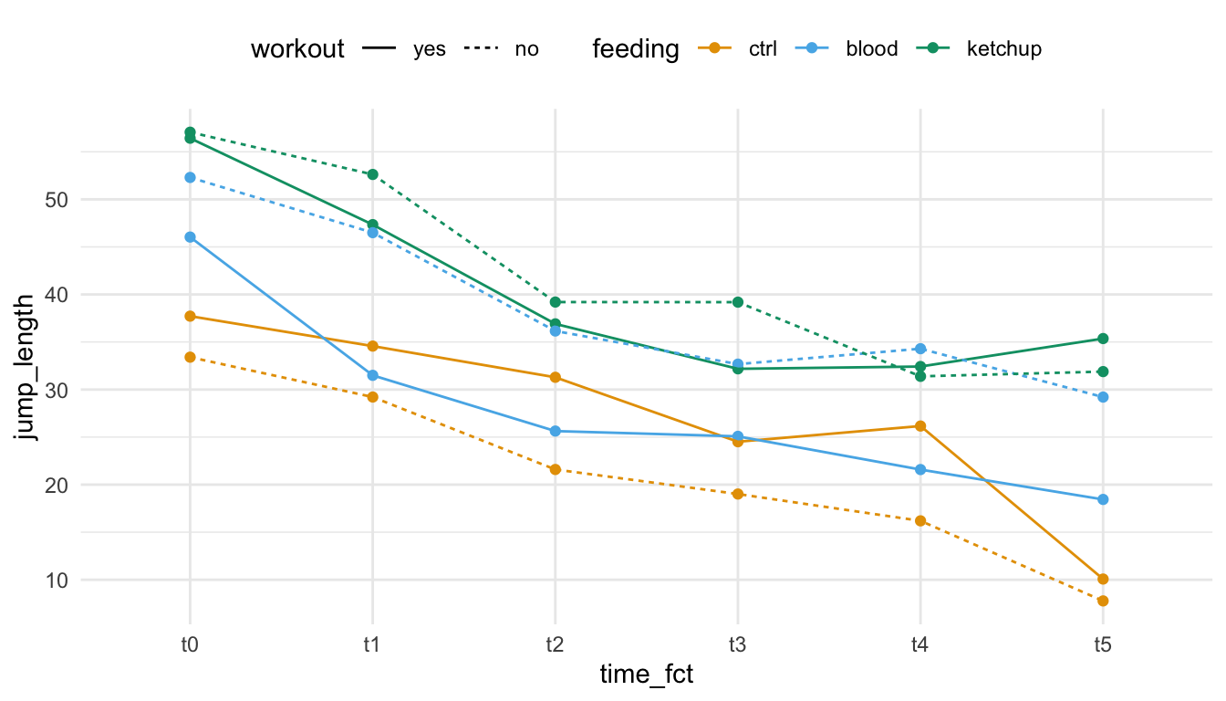
feeding sowie workout und time_fct. Die Linien sind in der Reichenfolge verdreht, es liegt eine Interaktion vor. Auch kruezen sich die Fütterungsarten über die Zeit. Eine allgmeine Aussage über die Sprungweite und die Fütterung soweie dem Workout lässt sich nicht unabhängig vom Zeitpunkt treffen.
34.5 Repeated measurement ANOVA
VorsichtAchtung, bitte beachten!
Willst du wirklich eine repeated ANOVA rechnen oder doch eher eine mixed ANOVA? Der Unterschied ist subtil und hängt davon ab, welche Behandlungskombinationen deine einzelnen Beobachtungen erhalten haben. Schaue im Zweifel nochmal oben in der Einleitung um dich zu versichern. Häufig möchtest du nämlich eine mixed ANOVA rechnen.
Schauen wir also einmal was die repeated ANOVA einmal macht. Hier nochmal ganz wichtig zu Anfang. Wir werden jetzte jede Beobachtung mit jeder Faktorkombination zu jedem Zeitpunkt messen. Das heißt in unserem Konkreten Fall, dass wir bei jeden Katzenfloh die Sprungweite zu jedem Zeitpunkt messen. Das macht ja auch erstmal Sinn. Das wäre dann die einfaktorielle repated ANOVA. Wir haben sonst auch keinen weiteren Faktor im Experiment. Wenn wir jetzt noch die Fütterungsart als Faktor hinzunehmen, dann füttern wir jeden Floh mit allen drei Arten der Fütterung. Jeder Floh erhält Zuckerwasser, springt dann mehrfach und wir messen die Sprungweite. Das machen wir dann mit dem selben Floh nochmal für die Ernährungsart Blut und Ketchup. Wenn dann noch ein zweiter Behandlungsfaktor hinzukommt wie das Workout, dann müssen wir unter jeder Workoutbedinung einmal alle drei Fütterungsarten die Sprungweiten für einen Floh durchmessen. Das heißt wir messen dann einen einzelnen Floh ganz schön oft. Im Bereich der Agrarwissenschaften mag diese Art der wiederholten Behandlung eher selten vorkommen. Daher hier auch ausdrücklich die Warnung, sich nochmal klar zu machen, wie du die einzelnen Beobachtungen nun bemisst. Ich habe auch erst ein wenig gebraucht um die repeated ANOVA von Design her zu verstehen.
34.5.1 Einfaktoriell
Beginnen wir mit der einfaktoriellen repeated ANOVA. Hier haben wir die Fragestellung vorliegen, ob die Zeit einen Einfluss auf die Sprungweiten der Katzenflöhe hat. Wir haben sonst keinen weiteren Behandlungsfaktor. Wir messen einfach nur die Sprungweite der Katzenflöhe wiederholt und schauen, ob sich die Sprungweiten über die Zeit ändern. Das Experiment ist eher ungewöhnlich, da wir hier ja nur wiederholt messen und sonst nichts tun. Faktisch ist es ein proof-of-principle, ob wir überhaupt einen Effekt der Zeit auf die Sprungweite haben.
Jetzt ist im Prinzip die Schreiweise das Besondere. Wir haben hier jetzt nur die Zeit als einen Einflussfaktor. Den packen wir jetzt einmal vorne in unser Modell und dann einmal hinten in den Fehlerterm. Dann müssen wir auch hier sagen, dass wir die Beobachtungen wiederholt im Faktor Zeit gemessen haben. Dann können wir auch schon die ANOVA rechnen.
R Code [zeigen / verbergen]
aov(jump_length ~ time_fct + Error(.id/time_fct), data = repeated_fac1_tbl)|>
  tidy() |>
  na.omit() |>
  select(term, df, statistic, p.value) |>
  mutate(p.value = pvalue(p.value))
# A tibble: 1 × 4
term df statistic p.value
<chr> <dbl> <dbl> <chr>
1 time_fct 3 19.1 <0.001 Wir sehen, dass der p-Wert kleiner ist als das Signifikanzniveau \(\alpha\) gleich 5% und damit haben wir einen signifkanten Einfluss der Zeit auf die Sprungweite der Katzenflöhe. Mehr testen wir hier auch nicht. Wir haben ja auch nur die Zeit als Faktor in unserem Modell.
Wenn du dann noch einen Effektschätzer brauchst, dann kannst du das R Paket {effectsize} mit der Funktion eta_squared() nutzen. Wir wollen dann noch das generalisierte Eta\(^2\) nutzen, da wir die Zeitpunkte nur beobachten und nicht als experimentellen Faktor festgelegt haben. Dazu dann auch mehr in der Arbeit von Olejnik & Algina (2003) mit dem Titel Generalized eta and omega squared statistics: measures of effect size for some common research designs.
R Code [zeigen / verbergen]
aov(jump_length ~ time_fct + Error(.id/time_fct), data = repeated_fac1_tbl) |>
  eta_squared(generalized = "time_fct")
# Effect Size for ANOVA (Type I)
Group | Parameter | Eta2 (generalized) | 95% CI
------------------------------------------------------------
.id:time_fct | time_fct | 0.46 | [0.22, 1.00]
- Observed variables: time_fct
- One-sided CIs: upper bound fixed at [1.00].Wir können auch das R Paket {rstatix} nutzen. Hier rufen wir am Ende dann doch auch nur die aov() Funktion auf, schreiben aber die Variablen in unseren Daten etwas anders in die Funkion anova_test(). Du musst eben wissen, dass hier die abhängige Variable dv die Sprungweite ist, du dann die Beobachtungen in wid schreibst und die Zeit in die Option within. Am Ende ist es dann auch hier eine Geschmackssache, welche Funktion dir besser gefällt und passt.
R Code [zeigen / verbergen]
rstatix_aov <- anova_test(data = repeated_fac1_tbl,
                          dv = jump_length, wid = .id, within = time_fct)
get_anova_table(rstatix_aov)
ANOVA Table (type III tests)
Effect DFn DFd F p p<.05 ges
1 time_fct 3 33 19.146 2.26e-07 * 0.465Es kommt das Gleiche numerisch raus, wie schon bei aov(). Wir erhalten hier aber zusätzlich noch einen Effektschätzer in der Spalte ges, was dem Eta\(^2\) entspricht. Demensprechend ein Vorteil der Funktion.
Das R Paket {afex} kommt bei einer so simplen einfaktoriellen repeated ANOVA dann auf die gleichen Zahlen wie schon die beiden vorherigen Algorithmen. Auch erhälst du bei der Funktion aov_car() einen Wert für Eta\(^2\) in der Spalte ges wiedergegeben. Ich bevorzuge dann ja die Schreibweise hier von {afex}, da ich diese hier etwas klarer finde als bei {rstatix}.
R Code [zeigen / verbergen]
aov_car(jump_length ~ time_fct + Error(.id/time_fct), data = repeated_fac1_tbl)Anova Table (Type 3 tests)
Response: jump_length
Effect df MSE F ges p.value
1 time_fct 2.68, 29.52 11.85 19.15 *** .465 <.001
---
Signif. codes: 0 '***' 0.001 '**' 0.01 '*' 0.05 '+' 0.1 ' ' 1
Sphericity correction method: GG Das R Paket {afex} erlaubt es auch die Modelle nach der Schreibweise der linearen gemischten Modelle zu definieren. Das ist für mich eigentlich etwas angenehmer, da man sich dann in einer Formelwelt aufhält mehr dazu dann im Kapitel zu gemischten Modellen. Also die Ergebnisse sind die Gleichen. Ich brauche es nur als Referenz für mich zum nachschlagen.
R Code [zeigen / verbergen]
aov_4(jump_length ~ time_fct + (time_fct|.id), data = repeated_fac1_tbl)Am Ende dann noch die Funktion RM() aus dem R Paket. Erstmal erhalten wir auch hier weder drei statistische Tests, obwohl wir nur nach einem gefragt haben. Ich würde auch hier nur die Ausgabe von ANOVA-Type Statistic (ATS) betrachten. Auch hier sehen wir, dass wir in einem einfaktoriellen Fall die gleichen Werte wie in den anderen R Paketen erhalten. Hir haben wir dann aber noch mehr Informationen, die wir dann brauchen oder auch nicht.
R Code [zeigen / verbergen]
RM(jump_length ~ time_fct, data = repeated_fac1_tbl,
   subject = ".id", within = "time_fct", iter = 100,
   resampling = "Perm", seed = 1234) |>
  summary()
Call:
jump_length ~ time_fct
A repeated measures analysis with 1 within-subject factor(s) ( time_fct ) and 0 between-subject factor(s).
Descriptive:
time_fct n Means Lower 95 % CI Upper 95 % CI
time_fct t1 12 24.081 22.212 25.950
time_fct.1 t2 12 30.642 28.189 33.096
time_fct.2 t3 12 28.107 24.974 31.239
time_fct.3 t4 12 21.410 18.982 23.838
Wald-Type Statistic (WTS):
Test statistic df p-value
time_fct "69.318" "3" "<0.001"
ANOVA-Type Statistic (ATS):
Test statistic df1 df2 p-value
time_fct "19.146" "2.684" "Inf" "<0.001"
p-values resampling:
Perm (WTS)
time_fct "<0.001" 34.5.2 Zweifaktoriell
Die zweifaktorielle repeated ANOVA wird jetzt schon interessanter. Wir haben jetzt nämlich neben der Zeit als Faktor noch eine Behandlung vorliegen. In unserem Beispiel erhält jeder Floh drei Arten der Fütterung wiederholt gefüttert. Zum einen erhält jeder Floh ein Zuckerwasser, dann Blut und zum Schluss Ketchup als Nahrung. Die Reihenfolge sollte sich dann von Floh Floh noch unterscheiden und die Zeiten zwischen den Behandlungen dann so lang gewählt werden, dass die Ernährung förmlich ausgewaschen ist. Die Idee ist, dass die vorherige Ernährungsform keinen Einfluss auf die neue Ernährung hat. Dann müssen wir das Ganze ja auch noch wiederholt über vier Zeitpunkte die Sprungweite messen. Daher misst du hier ganz schön viel. Häufig haben wir dieses Design nicht in den Agrarwissenschaften vorliegen. Wir können aber im Bereich der Nutztierwissenschaften schon das ein oder andere Mal so einen Fall vorliegen haben, wo wir Tiere wiederholt mit einer Behandlung verarzten.
Die Frage ist jetzt immer, wie schreibe ich jetzt das Modell richtig? Der komplizierte Teil ist eigentlich der Fehlerterm Error() aber auch der Teil davor. Ich nutze hier wieder die Kurzschreibweise mit dem Stern * um alle Faktorkombinationen plus Interaktion im Modell zu haben. Das wird eben dann ab zwei Faktoren etwas groß. So ist es dann weniger anfällig für Fehler. Dann musst du noch darauf achten, dass du in dem Fehlerterm die Klammern richtig setzt, sonst funktioniert es dort auch nicht. Erst kommt der Spaltenname für die einzelnen Flöhe .id und dahinter nach dem Slash / dann die Faktorkombinationen der Behandlungen und der Zeit. Dann räume ich die Ausgabe nochmal vollkommen auf, damit ich auch was sehe.
R Code [zeigen / verbergen]
aov(jump_length ~ feeding * time_fct + Error(.id/(feeding * time_fct)),
    data = repeated_fac2_tbl) |>
  tidy() |>
  na.omit() |>
  select(term, df, statistic, p.value) |>
  mutate(p.value = pvalue(p.value))
# A tibble: 3 × 4
term df statistic p.value
<chr> <dbl> <dbl> <chr>
1 feeding 2 151. <0.001
2 time_fct 3 64.7 <0.001
3 feeding:time_fct 6 9.48 <0.001 Wie wir sehen sind beide Faktoren der Zeit und der Fütterungsart signifikant. Der p-Wert ist kleiner als das Signifikanzniveau \(\alpha\) gleich 5%. Auch haben wir eine signifikante Interaktion zwischen den Fütterungsarten und der Zeit. Daher zeigen die Fütterungsarten unterschiedliche Sprungweiten zu den verschiedenen Zeitpunkten.
Dann können wir uns auch den Effektschätzer Eta^\(^2\) berechnen lassen. Hier müssen wir dann das ANOVA Modell einmal in die Funktion eta_squared() stecken und darauf achten, dass wir angeben, dass wir die Zeitpunkte nur beobachtet haben und nicht experimentell festgelegt. Deshalb kommt time_fct noch in die Option generalized mit rein. Die Effektschätzer unterscheiden sich hier immer ein wenig, dass kommt dann immer auf den verwendeten Algorithmus an.
R Code [zeigen / verbergen]
aov(jump_length ~ feeding * time_fct + Error(.id/(feeding * time_fct)),
    data = repeated_fac2_tbl) |>
  eta_squared(generalized = c("time_fct"))
# Effect Size for ANOVA (Type I)
Group | Parameter | Eta2 (generalized) | 95% CI
---------------------------------------------------------------------------
.id:feeding | feeding | 0.48 | [0.20, 1.00]
.id:time_fct | time_fct | 0.40 | [0.15, 1.00]
.id:feeding:time_fct | feeding:time_fct | 0.13 | [0.00, 1.00]
- Observed variables: time_fct
- One-sided CIs: upper bound fixed at [1.00].Das R Paket {rstatix} hat eine andere Schreibweise des Modells. Im Prinzip schreiben wir hier wieder nicht das Modell auf, sondern weisen die Spaltennamen dann den jeweiligen Optionen zu. Hier werden dann auch alle Interaktionen gerechnet, du kannst die Interaktionen aller Faktorkombinationen nicht abstellen. Wir setzten dann unseren Endpunkt jump_length in die Option dv und die einzelnen Beobachtungen in die Option wid. Dann müssen wir noch die beiden Faktoren der Zeit und der Behandlung in die Option within einfügen. Dann haben wir auch schon alles zusammen. Was hier etwas doof ist, ist das wir hier die Formelschreibweise in R verlassen, die wir dann aber überall sonst nutzen. Dafür erhalten wir dann aber das Eta\(^2\) gleich als ges wieder aus der Funktion zurück.
R Code [zeigen / verbergen]
rstatix_aov <- anova_test(data = repeated_fac2_tbl,
                          dv = jump_length, wid = .id,
                          within = c(feeding, time_fct))
get_anova_table(rstatix_aov)
ANOVA Table (type III tests)
Effect DFn DFd F p p<.05 ges
1 feeding 2 22 150.881 1.43e-13 * 0.667
2 time_fct 3 33 64.693 6.57e-14 * 0.459
3 feeding:time_fct 6 66 9.480 1.69e-07 * 0.216Wir erhalten die gleichen Ergebnisse wie schon bei der Funktion aov() wiedergegeben. Das überrascht auch nicht, den die Berechnung ist ja die gleiche Berechnung wie auch in aov() nur eben dann mit einem anderen Funktionsaufruf.
Das R Paket {afex} nutzt die Formelschreibweise und kann auch genau so bedient werden wie schon die Funktion aov(). Dafür können wir aber mit der Option type auch anderen Typen der ANOVA nutzen und nicht nur die Type I ANOVA in aov(). Das ist eigentlich die große Stärke von dem R Paket {afex}, dass wir hier flexibel bei der Auswahl der Typen sind. Bei der einfaktoriellen ANOVA war es noch egal, aber hier macht es mit zwei Faktoren dann schon einen Unterschied welche Art der ANOVA du rechnen möchtest. Ich nutze hier den Standard und damit die Type III ANOVA. Auch erhälst du bei der Funktion aov_car() einen Wert für Eta\(^2\) in der Spalte ges wiedergegeben.
R Code [zeigen / verbergen]
aov_car(jump_length ~ feeding * time_fct + Error(.id/feeding * time_fct),
        data = repeated_fac2_tbl)
Anova Table (Type 3 tests)
Response: jump_length
Effect df MSE F ges p.value
1 feeding 1.84, 20.24 18.95 150.88 *** .667 <.001
2 time_fct 2.43, 26.71 14.23 64.69 *** .459 <.001
3 feeding:time_fct 3.94, 43.39 19.43 9.48 *** .216 <.001
---
Signif. codes: 0 '***' 0.001 '**' 0.01 '*' 0.05 '+' 0.1 ' ' 1
Sphericity correction method: GG Die Ergebnisse sind ähnlich wie schon bei den beiden anderen Algorithmen, aber hier macht es dann einen Unterschied welche ANOVA grechnet wird. Wir rechnen hier dann ja eine Type 3 ANOVA. Die p-Werte sind aber alle so gering, dass es dann am Ende keinen so großen Unterschied mehr macht.
Das R Paket {afex} erlaubt es auch die Modelle nach der Schreibweise der linearen gemischten Modelle zu definieren. Das ist für mich eigentlich etwas angenehmer, da man sich dann in einer Formelwelt aufhält mehr dazu dann im Kapitel zu gemischten Modellen. Also die Ergebnisse sind die Gleichen. Ich brauche es nur als Referenz für mich zum nachschlagen.
R Code [zeigen / verbergen]
aov_4(jump_length ~ feeding * time_fct + (feeding * time_fct|.id),
      data = repeated_fac2_tbl)
Am Ende dann noch die Funktion RM() aus dem R Paket. Erstmal erhalten wir auch hier weder drei statistische Tests, obwohl wir nur nach einem gefragt haben. Ich würde auch hier nur die Ausgabe von ANOVA-Type Statistic (ATS) betrachten. Auch hier sehen wir, dass wir in einem zweifaktoriellen Fall die ähnlichen Werte wie in den anderen R Paketen erhalten. Hier fängt es dann etwas an zu variieren. Hier haben wir dann aber noch mehr Informationen, die wir dann brauchen oder auch nicht. Ich habe dann einmal hier die Anzeige der Funktion ausgeschaltet, da hier der Output dann sehr lang wird. Du kannst dir beispielhaft die Ausgabe einmal bei der einfaktoriellen repeated ANOVA weiter oben einmal anschaue oder eben den Code selber einmal durchführen.
R Code [zeigen / verbergen]
RM(jump_length ~ feeding * time_fct, data = repeated_fac2_tbl,
   subject = ".id", within = c("feeding", "time_fct"), iter = 100,
   resampling = "Perm", seed = 1234) |>
  summary()
34.5.3 Dreifaktoriell
Als letztes betrachten wir einen sehr exotischen Fall im Bereich der Agrarwissenschaften. Auch in anderen Forschungsbereichen ist die dreifaktorielle repeated ANOVA eher selten bis nicht vorhanden. Warum ist das so? Zum einen haben wir ja wieder unseren Faktor der Zeit. Wir messen hier viermal die Sprungweite eines Katzenflohs. Da wir aber dann noch zusätzlich zu dem Faktor der Zeit zwei weitere Behandlungen haben, kommen wir auf eine große Anzahl an Faktorkombinationen, die jeder Floh wiederholt durchlaufen muss. In unserem Fall haben wir ja die drei Fütterungsarten mit Zuckerwasser als Kontrolle, dem Blut sowie Ketchup als Ernährung. Dazu kommt dann noch ein Workout, dass jeder Floh gemacht hat oder nicht. Daher muss für jeden Floh jede Kombination der Fütterungsart und des Workouts wiederholt die Sprungweite gemessen werden. Das führt zu einem enormen Aufwand. Zum einen musst du ja immer Pausen zwischen den Behandlungen machen, damit sich die Effekte wieder auswaschen und es mit einem frischen Floh losgehen kann. Das ist eine zeitliche Belastung. Zum anderen ist es natürlich auch so, dass über die Zeit eventuell ein Floh nicht mehr kann oder gar verstirbt. Dann ist die ganze Messreihe für den Floh obsolet. Du siehst, diese Form des experimentellen Designs ist eher selten in Abschlussarbeiten und kommt eher in klinischen Studien oder längerfristigen agrarwissenschaftlichen Experimenten vor.
Die Frage ist jetzt immer, wie schreibe ich jetzt das Modell richtig? Der komplizierte Teil ist eigentlich der Fehlerterm Error() aber auch der Teil davor. Ich nutze hier wieder die Kurzschreibweise mit dem Stern * um alle Faktorkombinationen plus Interaktion im Modell zu haben. Das wird eben dann ab schon zwei Faktoren etwas groß und mit drei Faktoren sehr unübersichtlich. So ist es dann weniger anfällig für Fehler. Dann musst du noch darauf achten, dass du in dem Fehlerterm die Klammern richtig setzt, sonst funktioniert es dort auch nicht. Erst kommt der Spaltenname für die einzelnen Flöhe .id und dahinter nach dem Slash / dann die Faktorkombinationen der Behandlungen und der Zeit. Dann räume ich die Ausgabe nochmal vollkommen auf, damit ich auch was sehe.
R Code [zeigen / verbergen]
aov(jump_length ~ feeding * workout * time_fct +
      Error(.id/(feeding * workout * time_fct)),
    data = repeated_fac3_tbl) |>
  tidy() |>
  na.omit() |>
  select(term, df, statistic, p.value) |>
  mutate(p.value = pvalue(p.value))
# A tibble: 7 × 4
term df statistic p.value
<chr> <dbl> <dbl> <chr>
1 feeding 2 781. <0.001
2 workout 1 1000. <0.001
3 time_fct 3 84.2 <0.001
4 feeding:workout 2 2.87 0.078
5 feeding:time_fct 6 52.3 <0.001
6 workout:time_fct 3 0.472 0.704
7 feeding:workout:time_fct 6 0.873 0.520 Wir erhalten jetzt eine Menge an Ausgabe wieder. Insbesondere die vielen Interaktionen führen natürlich zu mehr Ausgabe. Aber auch hier sind erstmal die Haupteffekte der Art der Fütterung und des Workout am interessantesten. Wir sehen hier, dass beide Faktoren signifikant sind, der p-Wert liegt unter dem Signifikanzniveau von \(\alpha\) gleich 5%. Wir haben dann auch eine signifikante Zeitkomponente. Daher werden sich die Sprungweiten auch über die Zeit ändern. Am Ende ist dann nur die Interaktion zwischen der Fütterungsart und der Zeit signifikant. Anscheinend verhalten sich die Fütterungsarten nicht gleich über alle Zeitpunkte hinweg.
Dann können wir noch die Effektschätzer Eta\(^2\) für alle Faktoren und deren Interaktionen berechnen. Ich habe dann auch hier aufgeräumt und die Eta\(^2\)-Werte einmal gerundet, damit du besser sehen kannst, welche der Werte überhaupt größer sind. Auch hier sehen wir dann, dass die Hauptfaktoren den größten Effekt haben, gefolgt von den Zeitpunkten und der Interaktion zwischen den Fütterungsarten und der Zeit.
R Code [zeigen / verbergen]
aov(jump_length ~ feeding * workout * time_fct +
      Error(.id/(feeding * workout * time_fct)),
    data = repeated_fac3_tbl) |>
  eta_squared(generalized = c("time_fct")) |>
  select(Parameter, Eta2_generalized) |>
  mutate(Eta2_generalized = round(Eta2_generalized, 2))
# Effect Size for ANOVA
Parameter | Eta2 (generalized)
---------------------------------------------
feeding | 0.45
workout | 0.51
time_fct | 0.38
feeding:workout | 0.01
feeding:time_fct | 0.26
workout:time_fct | 0.00
feeding:workout:time_fct | 0.00Das R Paket {rstatix} hat eine andere Schreibweise des Modells. Im Prinzip schreiben wir hier wieder nicht das Modell auf, sondern weisen die Spaltennamen dann den jeweiligen Optionen zu. Hier werden dann auch alle Interaktionen gerechnet, du kannst die Interaktionen aller Faktorkombinationen nicht abstellen. Wir setzten dann unseren Endpunkt jump_length in die Option dv und die einzelnen Beobachtungen in die Option wid. Dann müssen wir noch die beiden Faktoren der Zeit und der beiden Behandlungen in die Option within einfügen. Dann haben wir auch schon alles zusammen. Was hier etwas doof ist, ist das wir hier die Formelschreibweise in R verlassen, die wir dann aber überall sonst nutzen. Dafür erhalten wir dann aber das Eta\(^2\) gleich als ges wieder aus der Funktion zurück.
R Code [zeigen / verbergen]
rstatix_aov <- anova_test(data = repeated_fac3_tbl,
                          dv = jump_length, wid = .id,
                          within = c(feeding, workout, time_fct))
get_anova_table(rstatix_aov)
ANOVA Table (type III tests)
Effect DFn DFd F p p<.05 ges
1 feeding 2 22 781.468 3.69e-21 * 0.700
2 workout 1 11 999.674 3.76e-12 * 0.749
3 time_fct 3 33 84.199 1.52e-15 * 0.518
4 feeding:workout 2 22 2.874 7.80e-02 0.018
5 feeding:time_fct 6 66 52.306 3.41e-23 * 0.428
6 workout:time_fct 3 33 0.472 7.04e-01 0.003
7 feeding:workout:time_fct 6 66 0.873 5.20e-01 0.013Wir erhalten die gleichen Ergebnisse wie schon bei der Funktion aov() wiedergegeben. Das überrascht auch nicht, den die Berechnung ist ja die gleiche Berechnung wie auch in aov() nur eben dann mit einem anderen Funktionsaufruf.
Das R Paket {afex} nutzt die Formelschreibweise und kann auch genau so bedient werden wie schon die Funktion aov(). Dafür können wir aber mit der Option type auch anderen Typen der ANOVA nutzen und nicht nur die Type I ANOVA in aov(). Das ist eigentlich die große Stärke von dem R Paket {afex}, dass wir hier flexibel bei der Auswahl der Typen sind. Bei der einfaktoriellen ANOVA war es noch egal, aber hier macht es mit zwei Faktoren dann schon einen Unterschied welche Art der ANOVA du rechnen möchtest. Ich nutze hier den Standard und damit die Type III ANOVA. Auch erhälst du bei der Funktion aov_car() einen Wert für Eta\(^2\) in der Spalte ges wiedergegeben.
R Code [zeigen / verbergen]
aov_car(jump_length ~ feeding * workout * time_fct +
          Error(.id/feeding * workout * time_fct),
        data = repeated_fac3_tbl)
Anova Table (Type 3 tests)
Response: jump_length
Effect df MSE F ges p.value
1 feeding 1.65, 18.15 10.60 781.47 *** .700 <.001
2 workout 1, 11 17.54 999.67 *** .749 <.001
3 time_fct 2.68, 29.52 27.90 84.20 *** .518 <.001
4 feeding:workout 1.71, 18.84 21.94 2.87 + .018 .088
5 feeding:time_fct 3.96, 43.61 21.16 52.31 *** .428 <.001
6 workout:time_fct 2.54, 27.91 15.60 0.47 .003 .674
7 feeding:workout:time_fct 3.57, 39.22 24.44 0.87 .013 .479
---
Signif. codes: 0 '***' 0.001 '**' 0.01 '*' 0.05 '+' 0.1 ' ' 1
Sphericity correction method: GG Die Ergebnisse sind ähnlich wie schon bei den beiden anderen Algorithmen, aber hier macht es dann einen Unterschied welche ANOVA grechnet wird. Wir rechnen hier dann ja eine Type 3 ANOVA. Die p-Werte sind aber alle so gering, dass es dann am Ende keinen so großen Unterschied mehr macht.
Das R Paket {afex} erlaubt es auch die Modelle nach der Schreibweise der linearen gemischten Modelle zu definieren. Das ist für mich eigentlich etwas angenehmer, da man sich dann in einer Formelwelt aufhält mehr dazu dann im Kapitel zu gemischten Modellen. Also die Ergebnisse sind die Gleichen. Ich brauche es nur als Referenz für mich zum nachschlagen.
R Code [zeigen / verbergen]
aov_4(jump_length ~ feeding * workout * time_fct +
        (feeding * workout * time_fct|.id),
      data = repeated_fac3_tbl)
Am Ende dann noch die Funktion RM() aus dem R Paket. Erstmal erhalten wir auch hier weder drei statistische Tests, obwohl wir nur nach einem gefragt haben. Ich würde auch hier nur die Ausgabe von ANOVA-Type Statistic (ATS) betrachten. Auch hier sehen wir, dass wir in einem dreifaktoriellen Fall die ähnlichen Werte wie in den anderen R Paketen erhalten. Je mehr Faktoren wir haben desto stärker werden dann auch die Unterschiede, da natürlich auch mehr Parameter geschätzt werden müssen. Hier haben wir dann aber noch mehr Informationen, die wir dann brauchen oder auch nicht. Ich habe dann einmal hier die Anzeige der Funktion ausgeschaltet, da hier der Output dann sehr lang wird. Du kannst dir beispielhaft die Ausgabe einmal bei der einfaktoriellen repeated ANOVA weiter oben einmal anschauen oder eben den Code selber einmal durchführen.
R Code [zeigen / verbergen]
RM(jump_length ~ feeding * workout * time_fct, data = repeated_fac3_tbl,
   subject = ".id", within = c("feeding", "workout", "time_fct"), iter = 100,
   resampling = "Perm", seed = 1234) |>
  summary()
Damit haben wir es dann auch geschafft. Was ist noch kommt sind die Anwendungsbeispiele in der mixed ANOVA. Ich habe noch keine Daten für eine repeated ANOVA bei mir liegen, daher warte ich hier mal ab, was noch kommt. Die beiden Beispiele zeigen aber einmal schön wie du eine zweifaktorielle mixed ANOVA rechnen kannst sowie eine dreifaktorielle mixed ANOVA. In beiden Fällen habe ich dann noch den Posthoc-Test in {emmeans} ergänzt. Ich nutze hier einmal die Funktionen aus dem R Paket {afex} aber du kannst auch ein anderes Paket oder aov() nutzen.
TippAnwendungsbeispiel: Gurkenwachstum (2-faktorielle mixed ANOVA)
In diesem beispiel wollen wir uns einmal das Gurkenwachstum anschauen. Wir haben dazu drei Gurkensorten Proloog, Quarto und Katrina vorliegen. Wir lassen jeweils sechs Gurken pro Sorte über vierzehn Wochen wachsen. Wir messen dabei jede Woche einmal die Länge von Gurken sowie deren Durchmesser. Hier kommt natürlich die Frage auf, welche Gurken messen wir eigentlich und so eine Pflanze hat ja auch mehrere Gurken. Das lassen wir hier mal im Raum stehen, wir haben einfach eine Gurken, die immer länger werden. Wir laden erstmal die Daten ein und nehmen aber nur die Sorten group und die Messzeitpunkte mit in die Analyse.
R Code [zeigen / verbergen]
gurke_tbl <- read_excel("data/wachstum_gurke.xlsx") |>
  clean_names() |>
  select(group = versuchsgruppe, t1:t14) |>
  mutate(group = as_factor(group))
In der folgenden Tabelle siehst du dann nochmal einen Ausschnitt aus den Daten. Wir werden jetzt gleich nur nach der Länge L filtern und auch die Daten aus dem Wide-Format in das Long-Format überführen.
t1 bis t4 dargestellt.
| group | t1 | t2 | t3 | t4 |
|---|---|---|---|---|
| Proloog L | 5.5 | 6.1 | 7.4 | 8.9 |
| Proloog L | 4.6 | 5.1 | 6.4 | 5.7 |
| Proloog L | 5.3 | 5.8 | 6.8 | 8.3 |
| ... | ... | ... | ... | ... |
| Katrina D | 0.86 | 0.87 | 0.9 | 1.1 |
| Katrina D | 0.62 | 0.67 | 0.7 | 0.71 |
| Tageslänge | 13.98 | 14.05 | 14.12 | 14.18 |
Die Längen werden mit einem L hinter dem Sortennamen angezeigt und der Durchmesser mit einem D hinter der Sorte. Deshalb filtern wir hier gleich mal nur die Daten mit den Gurkenlängen raus. Dann bauen wir uns noch einen Faktor mit den entsprechenden Namen. Die Daten brauchen wir noch im Long-Format und dazu nutze ich dann die Funktion pivot_longer(). Am Ende möchte ich immer nochmal die Zeitpunkte als Faktor sowie numerisch. Manchmal ist das eine einfacher in {ggplot} abzubilden als das andere.
R Code [zeigen / verbergen]
gurke_time_len_tbl <- gurke_tbl |>
  filter(str_detect(group, "L$")) |>
  rownames_to_column(".id") |>
  mutate(group = factor(group, labels = c("Proloog", "Quarto", "Katrina"))) |>
  pivot_longer(cols = t1:t14,
               values_to = "length",
               names_to = "time") |>
  mutate(time_fct = as_factor(time),
         time_num = as.numeric(time_fct)) |>
  filter(length != 0)
Dann kommen wir auch schon zur visuellen Darstellung der Daten. Hier habe ich dann einmal über alle vierzehn Zeitpunkte die mittlere Länge sowie die mediane Länge dargestellt. Die einzelnen Punkte stellen die einzelnen Beobachtungen dar. Hier fällt auf, dass eventuell einzelne Gurken eine etwas seltsames Längenwachstum haben. Wir würden ja davon ausgehen, dass eine Gurke wächst über die Zeit und nicht schrumpft. Am Ende sehen wir noch, dass die letzten Wochen nicht mehr vollständig bemessen wurden. Hier mag es dann Sinn machen, die letzten Wochen bis Woche t12 zu entfernen. Dann haben wir einen besseren Datensatz.
R Code [zeigen / verbergen]
ggplot(gurke_time_len_tbl,
       aes(time_fct, length, color = group,
           group = group)) +
  theme_minimal() +
  geom_point2() +
  stat_summary(fun = "mean", geom = "line") +
  stat_summary(fun = "median", geom = "line", linetype = 2) +
  scale_color_okabeito() +
  theme(legend.position = "top")+
  labs(x = "Zeitpunkte der Messung", y = "Gurkenlänge [cm]",
       color = "Sorte")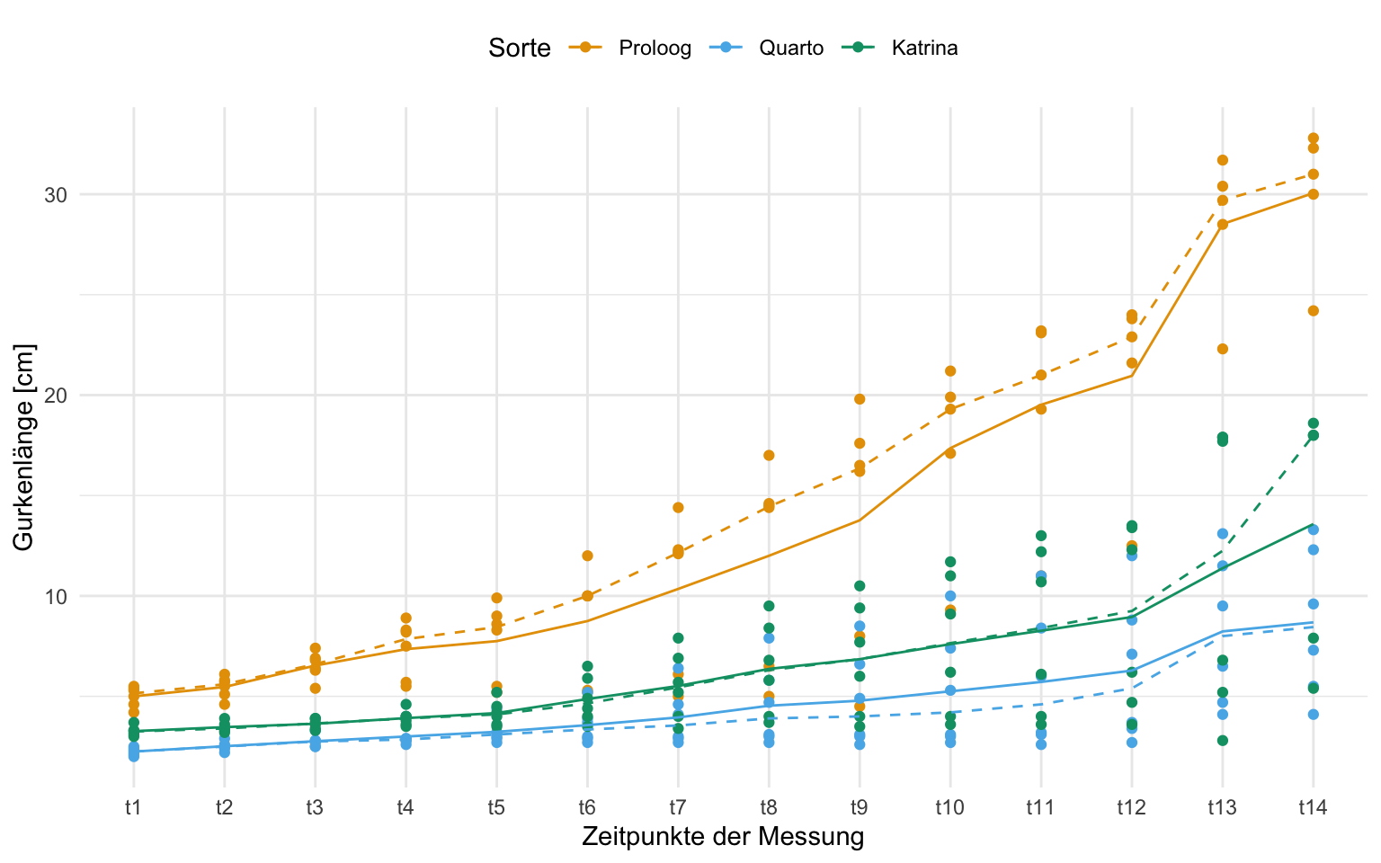
Um die einzelnen Gurkenpflanzen besser zu verstehen, habe ich einmal die Pflanzen einzeln als Verlauf über die Zeit dargestellt. Hier sehen wir dann wirklich einige seltsame Pflanzen. Ich habe hier nochmal über die Funktion geom_label_repel() die IDs der einzelnen Pflanzen zu den Verläufen ergänzt. Ich habe mir dann noch die Mühe gemacht, die Werte dann auch immer an den letzten Zeitpunkt zu schreiben. Wir sehen sehr schön, dass mit der Pflanze 2 irgendwas nicht stimmt. Die Gurkenpflanze 2 wächst nämlich nicht sondern schrumpft über die Zeit.
R Code [zeigen / verbergen]
max_time_tbl <- gurke_time_len_tbl |>
 group_by(group, .id) |>
  filter(time_num == max(time_num))

ggplot(gurke_time_len_tbl,
       aes(time_fct, log(length), color = group,
           group = .id)) +
  theme_minimal() +
  geom_point2() +
  geom_line(linetype = 11) +
  geom_label_repel(data = max_time_tbl, aes(time_fct, log(length), label = .id),
    box.padding = unit(0.35, "lines"), point.padding = unit(0.4, "lines"),
    segment.color = 'grey50', show.legend = FALSE) +
  scale_x_discrete(expand = expansion(mult = c(0, .1))) +
  scale_color_okabeito() +
  theme(legend.position = "top")+
  labs(x = "Zeitpunkte der Messung", y = "Gurkenlänge [cm] (log-scale)",
       color = "Sorte")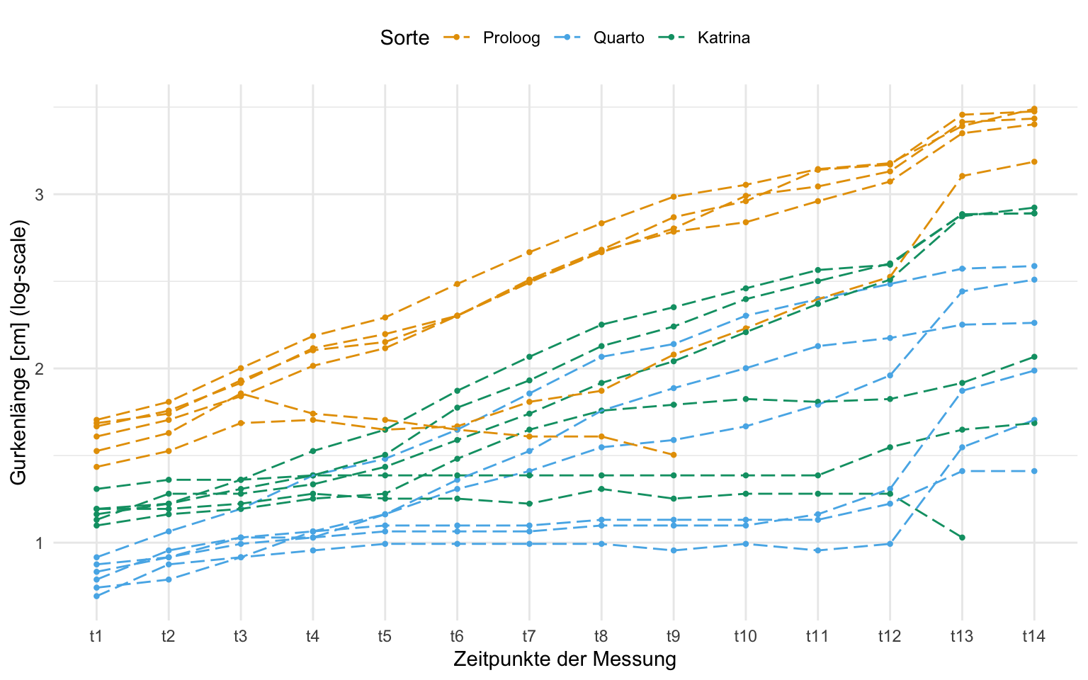
Dann können wir auch schon mit der Analyse der Daten mit einer mixed ANOVA beginnen. Je nachdem welche Schreibweise der Modelle in der ANOVA du bevorzugst, kannst du zwischen den beiden Funktionen aov_car() und aov_4() wählen. Ich habe hier für mich beide Formen einmal dargestellt. In beiden Fällen kommt das Gleiche raus, es geht eben nur um die Form der Darstellung der Modelle.
In dem Modell für R {base} nutzen wir die Schreibweise mit der Funktion Error() um den Fehlerterm und die Abhängigkeiten in dem Fehlerterm anzugeben. Hier haben wir die einzelnen Beobachtungen .id wiederholt in den Messzeitpunkten time_fct gemessen.
R Code [zeigen / verbergen]
aov_car(length ~ group * time_fct + Error(.id/time_fct),
        data = gurke_time_len_tbl)
Anova Table (Type 3 tests)
Response: length
Effect df MSE F ges p.value
1 group 2, 13 74.07 25.08 *** .704 <.001
2 time_fct 1.39, 18.11 33.11 92.69 *** .732 <.001
3 group:time_fct 2.79, 18.11 33.11 15.46 *** .477 <.001
---
Signif. codes: 0 '***' 0.001 '**' 0.01 '*' 0.05 '+' 0.1 ' ' 1
Sphericity correction method: GG Was sehen wir? Alle Faktoren und die Interaktion sind signifikant, da der p-Wert kleiner ist als das Signifikanzniveau \(\alpha\) gleich 5%. Im Weiteren sehen wir auch, dass die Effekte in der Spalte ges als Eta\(^2\) für die Versuchsgruppen sowie für die Zeit stark sind. Auch die Interaktion hat einen bedeutenden Effekt. Das wundert uns nicht, da wir ja Gurken haben, die über die Zeit weniger wachsen als alle anderen Gurken. Die Interaktion siehst du dann ganz gut an der Gurke Nr. 2 sowie an anderen Gurken gegen Ende der Untersuchung.
In dem Modell für R nach dem R Paket {lme4} und anderen Paketen nutzen wir die Schreibweise mit den Klammern () und dem Strich | um den Fehlerterm und die Abhängigkeiten in dem Fehlerterm anzugeben. Hier haben wir die einzelnen Beobachtungen .id wiederholt in den Messzeitpunkten time_fct gemessen.
R Code [zeigen / verbergen]
aov_4(length ~ group * time_fct + (time_fct|.id),
      data = gurke_time_len_tbl)
Anova Table (Type 3 tests)
Response: length
Effect df MSE F ges p.value
1 group 2, 13 74.07 25.08 *** .704 <.001
2 time_fct 1.39, 18.11 33.11 92.69 *** .732 <.001
3 group:time_fct 2.79, 18.11 33.11 15.46 *** .477 <.001
---
Signif. codes: 0 '***' 0.001 '**' 0.01 '*' 0.05 '+' 0.1 ' ' 1
Sphericity correction method: GG Für die Interpretation bitte den Tab zu der Funktion aov_car() beachten. Die Ausgaben sind die gleichen numerischen Werte und da beschreibe ich das für dich dann nur einmal.
Am Ende wollen wir dann noch die paarweisen Vergleich in {emmeans} rechnen. Dazu können wir dann direkt das Modell aus aov_car() nutzen und uns alle paarweisen Vergleiche getrennt für die Zeitpunkte wiedergeben lassen. Ändere einfach den Stich | durch einen Stern *, wenn du über alle Zeitpunkte hinweg vergleichen willst.
Es kommt jetzt ein riesiger Wust an Ausgabe. Am Ende können wir dann aber an jedem Zeitpunkt schauen, ob sich die drei Linien voneinander unterscheiden. Wir hätten hier natürlich nochmal die Daten aufreinigen müssen. Die Aufreinigung würde dann aber hier das Beispiel im Umfang sprengen. Auch habe ich hier auf eine Adjustierung der p-Werte verzichtet. Deshalb hier nur einmal die schnelle Analyse.
R Code [zeigen / verbergen]
aov_car(length ~ group * time_fct + Error(.id/time_fct),
        data = gurke_time_len_tbl) |>
  emmeans(~ group | time_fct) |>
  cld(Letters = letters, adjust = "none")
time_fct = t1:
group emmean SE df lower.CL upper.CL .group
Quarto 2.25 0.142 13 1.94 2.56 a
Katrina 3.26 0.156 13 2.92 3.60 b
Proloog 5.08 0.156 13 4.74 5.42 c
time_fct = t2:
group emmean SE df lower.CL upper.CL .group
Quarto 2.52 0.154 13 2.18 2.85 a
Katrina 3.50 0.168 13 3.14 3.86 b
Proloog 5.54 0.168 13 5.18 5.90 c
time_fct = t3:
group emmean SE df lower.CL upper.CL .group
Quarto 2.77 0.195 13 2.34 3.19 a
Katrina 3.68 0.214 13 3.22 4.14 b
Proloog 6.56 0.214 13 6.10 7.02 c
time_fct = t4:
group emmean SE df lower.CL upper.CL .group
Quarto 3.00 0.337 13 2.27 3.73 a
Katrina 3.98 0.369 13 3.18 4.78 a
Proloog 7.68 0.369 13 6.88 8.48 b
time_fct = t5:
group emmean SE df lower.CL upper.CL .group
Quarto 3.23 0.452 13 2.26 4.21 a
Katrina 4.30 0.495 13 3.23 5.37 a
Proloog 8.20 0.495 13 7.13 9.27 b
time_fct = t6:
group emmean SE df lower.CL upper.CL .group
Quarto 3.57 0.653 13 2.16 4.98 a
Katrina 5.14 0.716 13 3.59 6.69 a
Proloog 9.46 0.716 13 7.91 11.01 b
time_fct = t7:
group emmean SE df lower.CL upper.CL .group
Quarto 3.95 0.864 13 2.08 5.82 a
Katrina 5.94 0.946 13 3.90 7.98 a
Proloog 11.42 0.946 13 9.38 13.46 b
time_fct = t8:
group emmean SE df lower.CL upper.CL .group
Quarto 4.53 1.150 13 2.04 7.02 a
Katrina 6.90 1.260 13 4.17 9.63 a
Proloog 13.40 1.260 13 10.67 16.13 b
time_fct = t9:
group emmean SE df lower.CL upper.CL .group
Quarto 4.78 1.320 13 1.93 7.63 a
Katrina 7.52 1.440 13 4.40 10.64 a
Proloog 15.62 1.440 13 12.50 18.74 b
time_fct = t10:
group emmean SE df lower.CL upper.CL .group
Quarto 5.25 1.500 13 2.01 8.49 a
Katrina 8.40 1.640 13 4.85 11.95 a
Proloog 17.36 1.640 13 13.81 20.91 b
time_fct = t11:
group emmean SE df lower.CL upper.CL .group
Quarto 5.72 1.690 13 2.08 9.36 a
Katrina 9.20 1.850 13 5.21 13.19 a
Proloog 19.52 1.850 13 15.53 23.51 b
time_fct = t12:
group emmean SE df lower.CL upper.CL .group
Quarto 6.28 1.730 13 2.56 10.01 a
Katrina 10.02 1.890 13 5.94 14.10 a
Proloog 20.96 1.890 13 16.88 25.04 b
time_fct = t13:
group emmean SE df lower.CL upper.CL .group
Quarto 8.23 1.930 13 4.06 12.41 a
Katrina 13.10 2.120 13 8.52 17.68 a
Proloog 28.52 2.120 13 23.94 33.10 b
time_fct = t14:
group emmean SE df lower.CL upper.CL .group
Quarto 8.68 1.890 13 4.59 12.77 a
Katrina 13.58 2.070 13 9.10 18.06 a
Proloog 30.06 2.070 13 25.58 34.54 b
Confidence level used: 0.95
significance level used: alpha = 0.05
NOTE: If two or more means share the same grouping symbol,
then we cannot show them to be different.
But we also did not show them to be the same.
TippAnwendungsbeispiel: Grünkohlhöhe (3-faktorielle mixed ANOVA)
Im nächsten Beispiel schauen wir uns einmal die Höhe von Grünkohl an. Wir haben hier zwei Arten von Lichtgabe sowie zwei Sorten vorliegen. Dann messen wir die Höhe des Grünkohls noch an sieben Terminen. Daher haben wir hier wirklich mal eine dreifaktorielle ANOVA vorliegen. Da unsere beiden Behandlungsfaktoren nur zwei Level haben, können wir hier fast auf einen Post-hoc Test verzichten. Wir brauchen den Post-hoc Test aber dann für die Vergleiche in den jeweiligen Zeitpunkten. Wir laden also unseren Datensatz und nehmen nur die Wachstumsdaten mit den sieben Zeitpunkten.
R Code [zeigen / verbergen]
kale_tbl <- read_excel("data/kale_time_height.xlsx") |>
  clean_names() |>
  select(light, variety, t1:t7) |>
  mutate(light = as_factor(light),
         variety = as_factor(variety))
Dann hier einmal der Auszug aus den Daten zu dem Wachstum des Grünkohls. Ich habe hier nur die ersten vier Zeitpunkte ausgewählt. Wir müssen dann gleich einmal die Daten von dem Wide-Format in das Long-Format überführen. Für die Betrachtung ist es natütlich so schöner.
t1 bis t4 dargestellt.
| light | variety | t1 | t2 | t3 | t4 |
|---|---|---|---|---|---|
| dark light | Nero di Toscana | 2.5 | 3.5 | 7 | 8.6 |
| dark light | Nero di Toscana | 3.3 | 3.6 | 5.5 | 10 |
| dark light | Nero di Toscana | 4.5 | 5.6 | 5.75 | 6 |
| ... | ... | ... | ... | ... | ... |
| bright light | Oldenbor | 2.4 | 4 | 6.25 | 8.7 |
| bright light | Oldenbor | 2 | 3.8 | 6 | 8.3 |
| bright light | Oldenbor | 3.8 | 4.2 | 7 | 8.5 |
Es fehlen in den Daten noch die IDs für die einzelnen Grünkohlpflanzen. Das holen wir dann durch die Funktion rownames_to_column() einmal nach. Dann müssen wir noch die Daten in das Long-Format mit der Funktion pivot_longer() überführen.
R Code [zeigen / verbergen]
kale_time_height_tbl <- kale_tbl |>
  rownames_to_column(".id") |>
  pivot_longer(cols = t1:t7,
               values_to = "height",
               names_to = "time") |>
  mutate(time_fct = as_factor(time),
         time_num = as.numeric(time_fct))
Dann schauen wir uns in der folgenden Abbildung einmal die individuellen Verläufe des Höhenwachstums der Grünkohlpflanzen an. Wir sehen, dass die Pflanzen sehr schön und gleichmäßig wachsen. Hier gibt es keine Pflanze, die besonders auffällt und daher selektiert werden müsste.
R Code [zeigen / verbergen]
ggplot(kale_time_height_tbl,
       aes(time_fct, height, color = light, linetype = variety,
           group = .id)) +
  theme_minimal() +
  geom_line() +
  scale_color_okabeito() +
  theme(legend.position = "top")+
  labs(x = "Zeitpunkte der Messung", y = "Höhe Grünkohl [cm]",
       color = "Licht", linetype = "Sorte")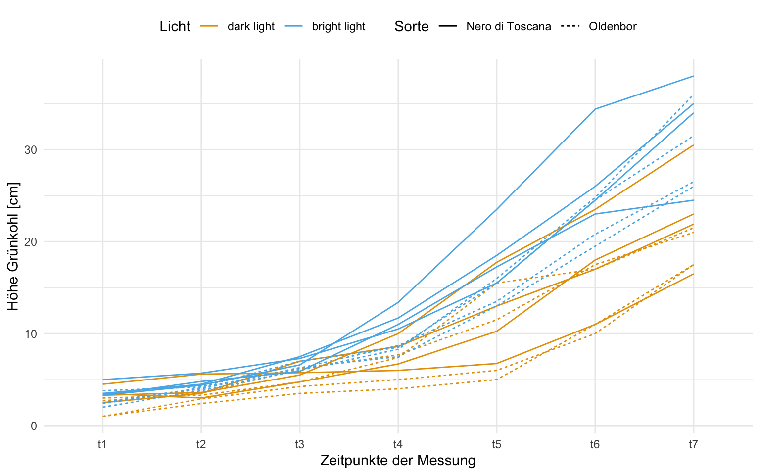
Nachdem wir die einzelnen Pflanzen angeschaut haben, können wir auch einmal für die vier Faktorkombinationen aus den zwei Lichtarten und den zwei Sorten einmal die Verläufe anschauen. Ich betrachte dann hier einmal die Mittelwerte. Wir sehen auch hier eine leichte Interaktion. Die Gerade laufen über die Zeit immer weiter auseinander. Auch sehen wir leichte Überschneidungen bei den ersten Zeitpunkten. Das mag dann auch zu einer signifikanten Interaktion führen.
R Code [zeigen / verbergen]
ggplot(kale_time_height_tbl,
       aes(time_fct, height, color = light, linetype = variety,
           shape = variety,
           group = interaction(light, variety))) +
  theme_minimal() +
  geom_point() +
  stat_summary(fun = "mean", geom = "line") +
  scale_color_okabeito() +
  theme(legend.position = "top")+
  labs(x = "Zeitpunkte der Messung", y = "Höhe Grünkohl [cm]",
color = "Licht", shape = "Sorte", linetype = "Sorte") 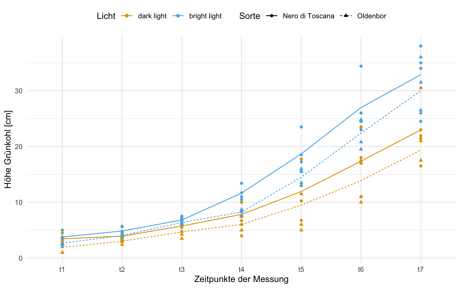
Dann können wir auch schon mit der Analyse der Daten mit einer mixed ANOVA beginnen. Je nachdem welche Schreibweise der Modelle in der ANOVA du bevorzugst, kannst du zwischen den beiden Funktionen aov_car() und aov_4() wählen. Ich habe hier für mich beide Formen einmal dargestellt. In beiden Fällen kommt das Gleiche raus, es geht eben nur um die Form der Darstellung der Modelle.
In dem Modell für R {base} nutzen wir die Schreibweise mit der Funktion Error() um den Fehlerterm und die Abhängigkeiten in dem Fehlerterm anzugeben. Hier haben wir die einzelnen Beobachtungen .id wiederholt in den Messzeitpunkten time_fct gemessen.
R Code [zeigen / verbergen]
aov_car(height ~ light * variety * time_fct + Error(.id/time_fct),
        data = kale_time_height_tbl)
Anova Table (Type 3 tests)
Response: height
Effect df MSE F ges p.value
1 light 1, 12 26.75 20.69 *** .430 <.001
2 variety 1, 12 26.75 5.55 * .168 .036
3 light:variety 1, 12 26.75 0.04 .001 .855
4 time_fct 1.58, 18.96 21.84 217.64 *** .911 <.001
5 light:time_fct 1.58, 18.96 21.84 11.12 ** .343 .001
6 variety:time_fct 1.58, 18.96 21.84 1.21 .054 .310
7 light:variety:time_fct 1.58, 18.96 21.84 0.20 .009 .768
---
Signif. codes: 0 '***' 0.001 '**' 0.01 '*' 0.05 '+' 0.1 ' ' 1
Sphericity correction method: GG Wenn wir die p-Werte betrachten, dann haben wir einen signifikanten Effekt der beiden Lichtarten. Die Sorten sind nur gerade noch so signifikant. Hier müsste man nochmal schauen, da der p-Wert doch recht nahe am Signifikanzniveau \(\alpha\) von 5% liegt. Die Zeit ist signifikant, aber das überrascht nicht, denn die Pflanzen wachsen ja über die Zeit. Es gibt keine Interaktion zwischen den beiden Hauptfaktoren. Dafür dann aber bei der Lichtart und der Zeit. Hier werden wir nochmal in extra nachschauen.
In dem Modell für R nach dem R Paket {lme4} und anderen Paketen nutzen wir die Schreibweise mit den Klammern () und dem Strich | um den Fehlerterm und die Abhängigkeiten in dem Fehlerterm anzugeben. Hier haben wir die einzelnen Beobachtungen .id wiederholt in den Messzeitpunkten time_fct gemessen.
R Code [zeigen / verbergen]
aov_4(height ~ light * variety * time_fct + (time_fct|.id),
      data = kale_time_height_tbl)
Anova Table (Type 3 tests)
Response: height
Effect df MSE F ges p.value
1 light 1, 12 26.75 20.69 *** .430 <.001
2 variety 1, 12 26.75 5.55 * .168 .036
3 light:variety 1, 12 26.75 0.04 .001 .855
4 time_fct 1.58, 18.96 21.84 217.64 *** .911 <.001
5 light:time_fct 1.58, 18.96 21.84 11.12 ** .343 .001
6 variety:time_fct 1.58, 18.96 21.84 1.21 .054 .310
7 light:variety:time_fct 1.58, 18.96 21.84 0.20 .009 .768
---
Signif. codes: 0 '***' 0.001 '**' 0.01 '*' 0.05 '+' 0.1 ' ' 1
Sphericity correction method: GG Für die Interpretation bitte den Tab zu der Funktion aov_car() beachten. Die Ausgaben sind die gleichen numerischen Werte und da beschreibe ich das für dich dann nur einmal.
Wir haben ja in der obigen Analyse eine signifikante Interaktion zwischen den Lichtarten und der Zeit gefunden. In der folgenden Abbildung will ich einmal anhand der Effektstärke schauen, wo die Interaktion herkommt. Ich entferne dafür immer einen weiteren Zeitpunkt aus der Analyse und schaue mir dann die Effektstärke Eta\(^2\) an. Du siehst sehr schön, dass die Interaktion unbedeutender wird, je weiter ich in der Zeit voranschreite. Die Interaktion liegt also eher in den frühen Zeitpunkten als in den späten Zeitpunkten vor. Das ist jetzt nicht so schlecht, da mich ja auch eher die späten Zeitpunkte interessieren. Das frühe Wachstum ist eher biologisch nicht so interessant.
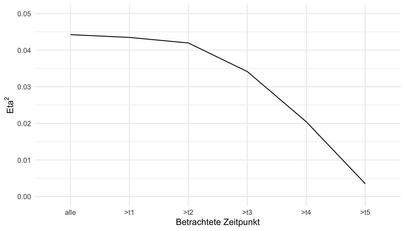
In unserem Fall ist der Posthoc-Test ja eigentlich mit nur zwei Lichtstärken und zwei Sorten nicht unbedingt nötig. Wenn du aber natürlich die Unterschiede für die einzelnen Zeitpunkte brauchst, dann kann dir hier {emmeans} helfen. Wir gehen hier von Varianzhomogenität in den Zeitpunkten aus. Dafür modellieren wir dann über alle Zeitpunkte hinweg die Varianz. Irgendwas ist ja immer. Hier kann man sicherlich noch weiter optimieren und mal bei den gemischten Modellen vorbeischauen, aber für die Anwendung reicht diese Auswertung auf jeden Fall aus.
R Code [zeigen / verbergen]
aov_car(height ~ light * variety * time_fct + Error(.id/time_fct),
        data = kale_time_height_tbl) |>
  emmeans(~ light * variety | time_fct, adjust = "none") |>
  cld(Letters = letters)
time_fct = t1:
light variety emmean SE df lower.CL upper.CL .group
dark light Oldenbor 1.93 0.441 12 0.963 2.89 a
bright light Oldenbor 2.67 0.441 12 1.713 3.64 a
dark light Nero di Toscana 3.45 0.441 12 2.488 4.41 a
bright light Nero di Toscana 3.77 0.441 12 2.813 4.74 a
time_fct = t2:
light variety emmean SE df lower.CL upper.CL .group
dark light Oldenbor 3.02 0.347 12 2.268 3.78 a
dark light Nero di Toscana 3.92 0.347 12 3.168 4.68 ab
bright light Oldenbor 4.03 0.347 12 3.268 4.78 ab
bright light Nero di Toscana 4.85 0.347 12 4.093 5.61 b
time_fct = t3:
light variety emmean SE df lower.CL upper.CL .group
dark light Oldenbor 4.67 0.425 12 3.750 5.60 a
dark light Nero di Toscana 5.75 0.425 12 4.825 6.68 ab
bright light Oldenbor 6.39 0.425 12 5.462 7.31 ab
bright light Nero di Toscana 6.83 0.425 12 5.900 7.75 b
time_fct = t4:
light variety emmean SE df lower.CL upper.CL .group
dark light Oldenbor 6.03 0.728 12 4.440 7.61 a
dark light Nero di Toscana 7.83 0.728 12 6.240 9.41 a
bright light Oldenbor 8.25 0.728 12 6.665 9.84 a
bright light Nero di Toscana 11.65 0.728 12 10.065 13.24 b
time_fct = t5:
light variety emmean SE df lower.CL upper.CL .group
dark light Oldenbor 9.50 1.930 12 5.291 13.71 a
dark light Nero di Toscana 11.94 1.930 12 7.729 16.15 ab
bright light Oldenbor 14.50 1.930 12 10.291 18.71 ab
bright light Nero di Toscana 18.69 1.930 12 14.479 22.90 b
time_fct = t6:
light variety emmean SE df lower.CL upper.CL .group
dark light Oldenbor 13.88 2.160 12 9.168 18.58 a
dark light Nero di Toscana 17.38 2.160 12 12.668 22.08 a
bright light Oldenbor 22.40 2.160 12 17.693 27.11 ab
bright light Nero di Toscana 26.98 2.160 12 22.268 31.68 b
time_fct = t7:
light variety emmean SE df lower.CL upper.CL .group
dark light Oldenbor 19.38 2.430 12 14.088 24.66 a
dark light Nero di Toscana 22.98 2.430 12 17.688 28.26 ab
bright light Oldenbor 30.00 2.430 12 24.713 35.29 b
bright light Nero di Toscana 32.88 2.430 12 27.588 38.16 b
Confidence level used: 0.95
P value adjustment: tukey method for comparing a family of 4 estimates
significance level used: alpha = 0.05
NOTE: If two or more means share the same grouping symbol,
then we cannot show them to be different.
But we also did not show them to be the same. Referenzen
Friedrich, S., Konietschke, F., & Pauly, M. (2019). Resampling-based analysis of multivariate data and repeated measures designs with the R package MANOVA. RM.
Gueorguieva, R., & Krystal, J. H. (2004). Move over anova: progress in analyzing repeated-measures data andits reflection in papers published in the archives of general psychiatry. Archives of general psychiatry, 61(3), 310–317.
Olejnik, S., & Algina, J. (2003). Generalized eta and omega squared statistics: measures of effect size for some common research designs. Psychological methods, 8(4), 434.