83 Baustelle
Letzte Änderung am 18. November 2025 um 19:34:21

VorsichtStand des Kapitels: Konstruktion (seit 07.2025)
Dieses Kapitel wird in den nächsten Wochen geschrieben. Ich plane zum Beginn des WiSe 2025/26 eine neue Version des Kapitels erstellt zu haben. Während das Kapitel entsteht, funktioniert so manches dann nicht so wie es soll.
VorsichtDieses Kapitel ist archiviert

Ich benötige die Thematik aktuell nicht in meiner Lehre oder der statistischen Beratung. Mir ist es als Nachschlagewerk aber immer noch wichtig zu behalten. Archivierte Kapitel werden nicht von mir weiter gepflegt oder ergänzt. Auftretende Fehler werden aber natürlich beseitigt, wenn die Fehler mir auffallen oder gemeldet werden.
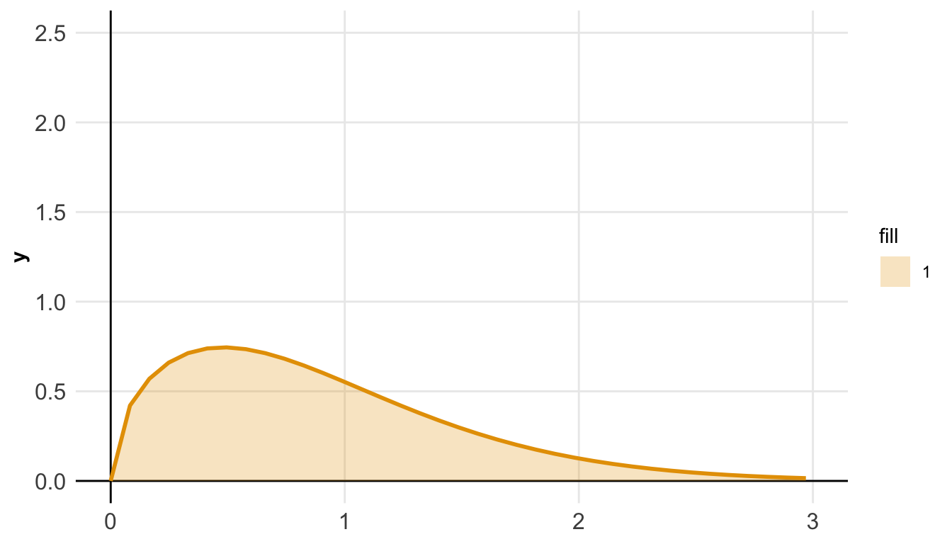
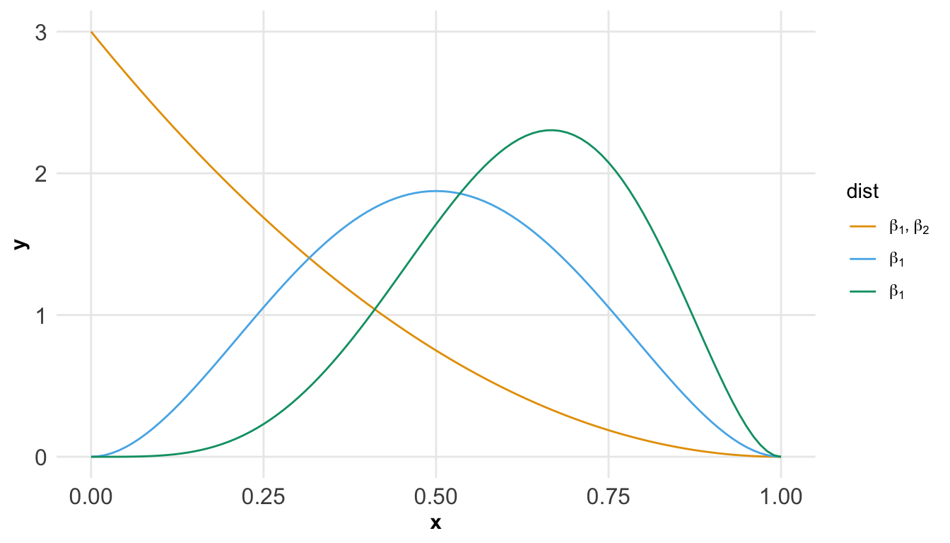
83.1 Visualisierung von Verteilungen
rnorm(): Erzeugt Zufallszahlen aus einer Normalverteilung.runif(): Erzeugt Zufallszahlen aus einer Gleichverteilung.rbinom(): Generiert Zufallszahlen aus einer Binomialverteilung.rpois(): Erzeugt Zufallszahlen aus einer Poisson-Verteilung.rgamma(): Generiert Zufallszahlen aus einer Gamma-Verteilung.rexp(): Erzeugt Zufallszahlen aus einer Exponentialverteilung.rt(): Generiert Zufallszahlen aus einer Student’s t-Verteilung.rchisq(): Erzeugt Zufallszahlen aus einer Chi-Quadrat-Verteilung.rbeta(): Erzeugt Zufallszahlen aus einer Beta-Verteilung.rf(): Erzeugt Zufallszahlen aus einer F-Verteilung.rlogis(): Erzeugt Zufallszahlen aus einer logistischen Verteilung.rweibull(): Erzeugt Zufallszahlen aus einer Weibull-Verteilung.
83.2 Daten generieren
R Code [zeigen / verbergen]
library(ggeffects)Warning: package 'ggeffects' was built under R version 4.4.1R Code [zeigen / verbergen]
set.seed(1234)
x <- rnorm(200, 5, 1)
z <- rnorm(200)
# quadratic relationship
# y <- 5 + 2 * x + x^2 + 4 * z + rnorm(200)
y <- 5 + 2 * (x-5) + (x-5)^2 + 4 * z + rnorm(200)
y <- x^2 - 8*x + 4*z +20 ## das war Gemini KI


d <- data.frame(x = x, y, z)
m <- lm(y ~ x + z, data = d)

pr <- predict_response(m, "x [all]")
p1 <- plot(pr, show_data = TRUE)
Data points may overlap. Use the `jitter` argument to add some amount of
random variation to the location of data points and avoid overplotting.R Code [zeigen / verbergen]
p2 <- plot(pr, show_residuals = TRUE, show_residuals_line = TRUE)Data points may overlap. Use the `jitter` argument to add some amount of
random variation to the location of data points and avoid overplotting.R Code [zeigen / verbergen]
p1 + p2`geom_smooth()` using formula = 'y ~ x'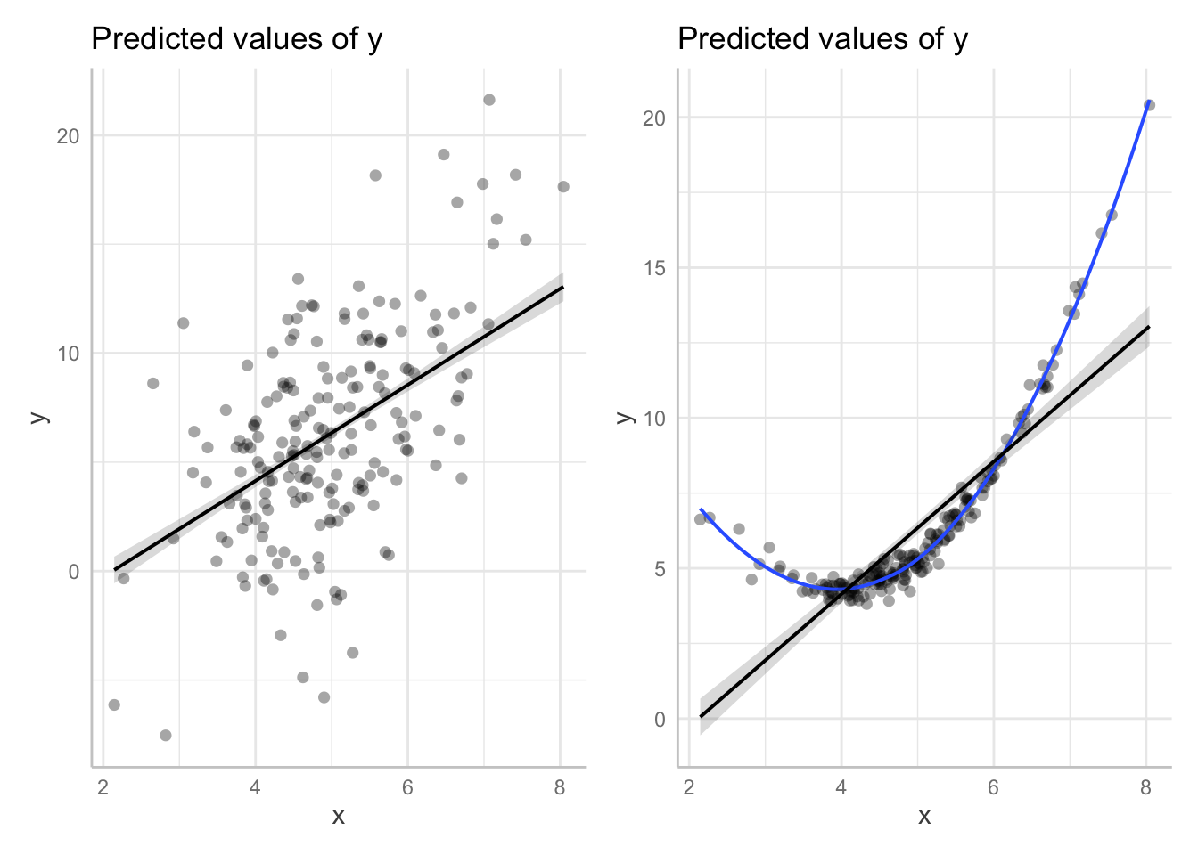
R Code [zeigen / verbergen]
x <- seq(-3, 3, length.out = 200) + rnorm(200) + 5
z <- rnorm(200)
y <- 5 + 2 * x + x^2 + x^3 + 4 * z + rnorm(200)
y <- 5 + 2 * (x-5) - (x-5)^2 + (x-5)^3 + 4 * z + rnorm(200)
y <- x^3 - 16*x^2 + 87*x + 4*z - 155

d <- data.frame(x = x, y, z)
m <- lm(y ~ x + z, data = d)

pr <- predict_response(m, "x [all]")
p1 <- plot(pr, show_data = TRUE)
Data points may overlap. Use the `jitter` argument to add some amount of
random variation to the location of data points and avoid overplotting.R Code [zeigen / verbergen]
p2 <- plot(pr, show_residuals = TRUE, show_residuals_line = TRUE)Data points may overlap. Use the `jitter` argument to add some amount of
random variation to the location of data points and avoid overplotting.R Code [zeigen / verbergen]
p1 + p2`geom_smooth()` using formula = 'y ~ x'
Introduction: Adding Partial Residuals to Adjusted Predictions Plots
83.2.1 … mit {modelbased}
83.3 Maximum Liklihood
83.4 Konfidenzintervall vs. Prädiktionsintervall
Ein Konfidenzintervall gibt den Wertebereich für einen gesuchten Parameter der Grundgesamtheit mit einer bestimmten Wahrscheinlichkeit an. Ein Prognoseintervall gibt den Wertebereich für einen individuellen, zukünftig zu beobachtenden Wert mit einer bestimmten Wahrscheinlichkeit an.
- Konfidenzintervall
-
Ein Konfidenzintervall gibt den Wertebereich für einen gesuchten Parameter der Grundgesamtheit mit einer bestimmten Wahrscheinlichkeit an.
- Prädiktionsintervall
-
Ein Prädiktionsintervall (auch Vorhersageintervall oder Prognoseintervall) gibt den Wertebereich für einen individuellen, zukünftig zu beobachtenden Wert mit einer bestimmten Wahrscheinlichkeit an.
Quantile Regression Forests for Prediction Intervals
The difference between prediction intervals and confidence intervals
P-values for prediction intervals machen keinen Sinn
83.5 Concordance Correlation Coefficient (CCC)
Kann auch in technische Gleichheit mit rein
R Code [zeigen / verbergen]
nirs_wide_tbl <- read_excel("data/nirs_qs_data.xlsx") |>
  clean_names()

nirs_long_tbl <- nirs_wide_tbl |>
  pivot_longer(cols = jd_ts:last_col(),
               values_to = "values",
               names_to = c("method", "type"),
               names_sep = "_") |>
  mutate(gulleart = as_factor(gulleart),
         method = as_factor(method),
         type = as_factor(type))
Warning: Expected 2 pieces. Additional pieces discarded in 3 rows [3, 8, 13].Technical note: Validation and comparison of 2 commercially available activity loggers
User’s guide to correlation coefficients
Concordance correlation coefficient calculation in R
How does Polychoric Correlation Work? (aka Ordinal-to-Ordinal correlation)
An Alternative to the Correlation Coefficient That Works For Numeric and Categorical Variables
83.6 Dummykodierung
R Library Contrast Coding Systems for categorical variables
fastDummies: Fast Creation of Dummy (Binary) Columns and Rows from Categorical Variables
83.7 Analyse von Zeitreihen mit {gamm4}
Hier nochmal {mgcv} und {gamm4}
Introduction to Generalized Additive Mixed Models
s() und Interaktion mit s(x_1, by = f_1)
83.8 Mediatoranalyse
Simulating confounders, colliders and mediators
Statistical Control Requires Causal Justification
Mediators, confounders, colliders – a crash course in causal inference
Collider Bias in Beobachtungsstudien: Konsequenzen für die medizinische Forschung
Thinking Clearly About Correlations and Causation: Graphical Causal Models for Observational Data
DAGitty — draw and analyze causal diagrams
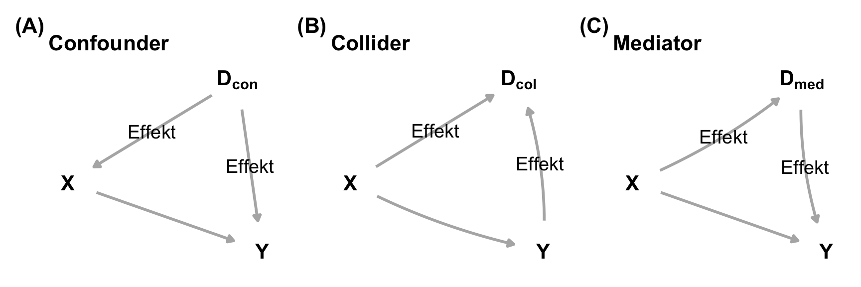
In dem Begriff des Disturber (deu. Störenfried, abk. \(D\)) fassen wir die Begriffe des Confounder (deu. Störfaktor, abk. \(D_{con}\)), Collider (deu. Zusammenstoßen, abk. \(D_{col}\)) und Mediator (deu. Vermittlern, abk. \(D_{med}\)) zusammen.
Structural Equation Modeling
Passt das hier rein? Müssen wir nochmal überlegen.
Van Lissa et al. (2023) tidySEM
Introduction to structural equation modeling (sem) in r with lavaan
Intro to structural equation modeling
Schöne Diagramme Structural Equation Models
Bayes Ideen
https://paul-buerkner.github.io/brms/articles/index.html
https://paul-buerkner.github.io/brms/articles/brms_nonlinear.html
https://bookdown.org/content/4857/
https://bayesat.github.io/lund2018/slides/andrey_anikin_slides.pdf
http://mjskay.github.io/tidybayes/articles/tidybayes.html
Half a dozen frequentist and Bayesian ways to measure the difference in means in two groups
https://bookdown.org/marklhc/notes_bookdown/group-comparisons.html
Van Lissa, C. J., Villarreal, M. G., & Anadria, D. (2023). Best Practices in Latent Class Analysis using the Open-Source R-Package tidySEM.