```{r echo = FALSE, warning = FALSE, message=FALSE}
source("init.R")
pacman::p_load(ggridges, ggbeeswarm, janitor, data.table, kableExtra, ggmosaic2,
               gtsummary)
conflicts_prefer(dplyr::select)

## gummy stats
gummy_tbl <- read_excel("data/gummibears.xlsx")
gummy_color_tbl <- gummy_tbl |>
  select(darkred:white) |>
  gather(color, count)
count_bears <- sum(gummy_color_tbl$count)
full_person <- gummy_tbl |> na.omit() |> nrow()
```

# Gummy bears {#sec-temp}

*Last modified on `r format(fs::file_info("interlude-I-gummibaers.qmd")$modification_time, '%d. %B %Y at %H:%M:%S')`*

> *"Gummy Bears! Bouncing here and there and everywhere; High adventure that's beyond compare; They are the Gummy Bears." --- Gummy Bears Theme, Adventures of the Gummy Bears*

This chapter provides a brief interlude to present an analysis of a dataset that I am personally connected to. If you work with data that you have generated, that data becomes very special. It's like the rose in The Little Prince. It is not just one of thousands of data sets. It is my data set. Like every other data set, this one has a special story behind it. Where there is a story, there are also emotions. Follow me on the path to truth, guided by gummy bears.

## General background

Like any good research story, this one begins in a gay club in Berlin with mirrored bathrooms, where you can see everything. Nothing stays hidden. When you can observe everything, no questions remain unanswered. This is somehow boring and not worthwhile for a truth-seeker. However, if you cannot see the truth before you, then you must draw conclusions based on your incomplete observations of reality.

There was a bag of gummy bears lying on the table. As the comedian performing this evening was from Scotland, I didn't understand much of what was said. Therefore, I focused on the bag. It had all six colours of bear. How disappointing. I asked myself, 'What is the probability of getting only one bag with the same colour?' Was it even possible? Or does Haribo, the company that produced these sweets, secretly rig the packing process so that there will always be a variety of colours and flavours in a bag?

Therefore, I started a survey in 2018. Had I ever imagined how long it would go on for, or how many gummy bears I would end up counting, I would have stopped immediately. However, I was unaware of this, so I created a simple spreadsheet in Google Spreadsheets, shared the shortened link with every new lecture I gave, and counted the number of gummy bears, as well as collecting some demographic data about the students. From the beginning, one idea was good: I only collected some demographic data, such as body height, age, and the most popular flavour of gummy bear. Therefore, the data is from real people, but is anonymised as much as possible.

While you are reading these lines, the dataset is still growing. Currently, we have $`r nrow(gummy_tbl)`$ bags containing $`r count_bears`$ bears, counted by $`r full_person`$ people. There are more bags of gummy bears than people who have counted them because some people counted the bears but did not enter any demographic information, or only entered it in part. Therefore, there is a lack of data. The beauty lies in the numbers: over one thousand bags and people, as well as over ten thousand bears counted in nearly ten years.

Therefore, we come to my urgent question. Given my average speed at counting bags during my lectures, is it possible that I will find a bag containing only one colour in my lifetime? Follow me through this chapter to find the answer!

## Theoretical background

## Data

I started generating data in 2028. From the beginning, the data generation process has been very hands-on and has not changed since. There is an empty Google spreadsheet with a shortened link. The process has not changed in any of the years that I have conducted the survey. First, I distribute the bags of gummy bears among the students. Each student gets one bag and can eat all the sweets after the survey. Then I present the link, and all the students join the same Google spreadsheet. Depending on the size of the lecture, it can get a little chaotic, but in the end, all the bears are counted and some demographic data is gathered.

The gummy bear data is split into two parts. The first part is a matrix showing the number of gummy bears of each of the six colours: dark red (d), light red (l), orange (o), yellow (y), green (g) and white (w). The second part shows the self-reported bear count and number of colours. Some errors can occur here. Because the bears and the number of colours have to be counted by the counter. Therefore, a discrepancy can occur between the colour matrix and the reported number of bears and colours. The second part includes some demographic information about the consumer. I wanted to know their age, height and favourite flavour of gummy bear.

### Characteristics of gummy bears

```{r}
#| echo: false
#| message: false
#| warning: false

gummy_tbl <- read_excel("data/gummibears.xlsx") |>
  mutate(gender = factor(gender, levels = c("w", "m"), labels = c("female", "male")))
```

```{r}
#| echo: false
#| message: false
#| warning: false
#| label: tbl-gummy-bears
#| tbl-cap: "Extract of the gummy bears dataset of the characteristics of gummy bears. The year of the survey is reported, as well as the number of bears of each colour that were counted. The last two columns show the self-reported bear and colour counts."

gummy_bears_tbl <- gummy_tbl |>
  select(year:count_color) |>
  rename(color_obs = count_color,
         bear_obs = count_bears)

rbind(head(gummy_bears_tbl, n = 3),
      rep("...", times = ncol(gummy_bears_tbl)),
      tail(gummy_bears_tbl, n = 3)) |>
  set_names(c("Year", "Dark red", "Light red", "Orange", "Yellow", "Green", "White", "Bears", "Colors")) |>
  kable(align = "c", "pipe") |>
  add_header_above(c(" " = 1, "Gummy bear color" = 6, "Observed" = 2))
```

```{r}
#| echo: false
gummy_count_tbl <- gummy_bears_tbl %>%
  rowwise() %>%
  mutate(bear_exp = sum(c_across(darkred:white)),
         color_exp = sum(c_across(darkred:white) > 0),
         bear_diff = bear_obs - bear_exp,
         color_diff = color_obs - color_exp) |>
  ungroup() |>
  select(year, bear_obs, bear_exp, bear_diff, color_obs, color_exp, color_diff)
```

```{r}
#| echo: false
#| message: false
#| warning: false
#| label: tbl-gummy-bears-count
#| tbl-cap: "Extract of the gummy bear dataset of the self-reported counts ('observed') of the number of gummy bears, as well as their colours, and the deviation from the calculated counts from the gummy bear colour matrix ('expected') separated for the year and individual counting person. Each line represents one bag."

rbind(head(gummy_count_tbl, n = 3),
      rep("...", times = ncol(gummy_count_tbl)),
      tail(gummy_count_tbl, n = 3)) |>
  set_names(c("Year", "Observed", "Expected", "Deviation", "Observed", "Expected", "Deviation")) |>
  kable(align = "c", "pipe") |>
  add_header_above(c(" " = 1, "Number of bears (b)" = 3, "Number of colors (c)" = 3))
```


```{r}
#| echo: false
#| message: false
#| warning: false
#| label: fig-chap-interlude-I-diff-2
#| fig-align: center
#| fig-height: 2.5
#| fig-width: 7
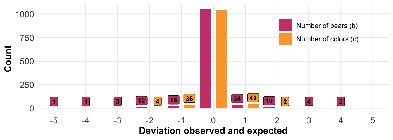
#| fig-cap: "Deviation between the sum of the gummy bear out of the count matrix and the self-reported counts of bears and colour in a bag. Most people deliver the same values; no deviation can be determined. The observed deviations scatter in both positive and negative directions. No bias can be observed. The following analysis uses the calculated and therefore expected values from the count matrix."

gummy_count_tbl |>
  select(bear_diff, color_diff) |>
  stack() |>
  mutate(ind = factor(ind, labels = c("Number of bears (b)", "Number of colors (c)"))) |>
  ggplot(aes(x = values, fill = ind)) +
  theme_book() +
  ## facet_wrap(~ ind, scale = "free_x") +
  geom_bar(position = position_dodge(1, preserve = "single"), width = 0.7) +
  geom_label(stat='count', aes(label=..count.., y = ..count.. +70), size = 3,
             position = position_dodge(1), show.legend = FALSE, fontface = 2) +
  scale_x_continuous(breaks = seq(-5, 5,1), limits = c(-5, 5)) +
  scale_y_continuous(breaks = seq(0, 1200, 250), limits = c(0, 1050)) +
  scale_fill_viridis(option = "plasma", discrete = TRUE, begin = 0.5, end = 0.8,
                     alpha = 1) +
  labs(x = "Deviation observed and expected", y = "Count", fill = "") +
  theme(legend.position = c(0.8, 0.8))
```

```{r}
#| echo: false
#| message: false
#| warning: false
#| label: tbl-gummy-color-exp
#| tbl-cap: "Expected colour counts in a bag and the corresponding counts in the survey in absolute numbers as well as the percentage."

lower_gummy_count_tbl <- gummy_count_tbl |>
janitor::tabyl(color_exp)

rbind(tibble(color_exp = 1, n = 0, percent = 0),
      lower_gummy_count_tbl) |>
  mutate(percent = scales::percent(round(percent, 4))) |>
  set_names(c("Expected colors (c)", "Number", "Percentage")) |>
  kable(align = "c", "pipe")
```

```{r}
#| echo: false
#| message: false
#| warning: false
#| label: tbl-gummy-bear-exp
#| tbl-cap: "Expected bear counts in a bag and the corresponding counts in the survey in absolute numbers as well as the percentage."

gummy_count_tbl |>
janitor::tabyl(bear_exp) |>
  mutate(percent = scales::percent(round(percent, 4))) |>
  set_names(c("Expected bears (b)", "Number", "Percentage")) |>
  kable(align = "c", "pipe")
```

### Characteristics of the counters

```{r}
#| echo: false
#| message: false
#| warning: false
#| label: tbl-gummy-sudent
#| tbl-cap: "Extract of the gummy bear dataset of the most liked taste of the gummy bear, the gender, the grouped age and the body height of each counting person. The age groups have been created based on the continuous reported ages from each survey year. All measures are self reported."

gummy_student_tbl <- gummy_tbl |>
  mutate(age_grp = case_when(age <= 21 ~ "<22",
                             age > 21 & age <= 29 ~ "22-29",
                             age >= 30 ~ "30+"),
         age_grp = factor(age_grp, levels = c("<22", "22-29", "30+"))) |>
  select(most_liked, gender, age_grp, height)

gummy_student_raw_tbl <- gummy_student_tbl |>
  mutate(gender = as.character(gender),
         age_grp = as.character(age_grp))

rbind(head(gummy_student_raw_tbl, n = 3),
      rep("...", times = ncol(gummy_student_raw_tbl)),
      tail(gummy_student_raw_tbl, n = 3)) |>
  set_names(c("Most liked taste", "Gender", "Grouped age", "Body height [cm]")) |>
  kable(align = "c", "pipe")
```


```{r}
#| echo: false
#| message: false
#| warning: false
#| label: tbl-gummy-sudent-tbl-summary
#| tbl-cap: "Information on the height, age and grouped age of the female and male gummy bear counters."

gummy_tbl |>
  mutate(age_grp = case_when(age <= 21 ~ "<22",
                             age > 21 & age <= 29 ~ "22-29",
                             age >= 30 ~ "30+"),
         age_grp = factor(age_grp, levels = c("<22", "22-29", "30+"))) |>
  select(height, age, age_grp, gender) |>
  tbl_summary(
    by = gender,
    statistic = list(
      all_continuous() ~ "{mean} ({sd})",
      all_categorical() ~ "{n} / {N} ({p}%)"
    ),
    digits = all_continuous() ~ 2,
    label = age_grp ~ "age group",
    missing_text = "(Missing)"
  )
```


## Results

### Gummy bears over the years of the survey

```{r}
#| echo: false
#| message: false
#| warning: false
#| label: fig-chap-interlude-I-count-bears-year
#| fig-align: center
#| fig-height: 3.5
#| fig-width: 7
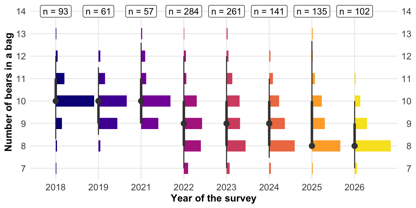
#| fig-cap: "Dependency of the number of bears in a bag and the year of the survey. Due to the pandemic, data for 2020 is missing. The number of counted bags is shown above the histogram. The point and interval indicate the median and the range of quantiles. A clear shrinkage in the size of the gummy bear bags can be observed over the years."

count_tbl <- gummy_count_tbl |>
  pull(year) |>
  janitor::tabyl()

gummy_count_tbl |>
  ggplot(aes(x = bear_exp, y = as_factor(year),
             fill = as_factor(year))) +
  theme_book() +
  ## stat_density_ridges() +
  stat_histinterval(breaks = breaks_fixed(width = 0.5),
                    align = align_center(at = 0), color = "gray25") +
  scale_x_continuous(breaks = seq(6, 15, by = 1), limits = c(6.5, 14),
                     sec.axis = sec_axis(~., breaks = seq(6, 15, by = 1)),
                     expand = expansion(mult = c(0, 0.04))) +
  labs(x = "Number of bears in a bag", y = "Year of the survey") +
  theme(legend.position = "none") +
  scale_fill_viridis(option = "plasma", discrete = TRUE, end = 0.95) +
  annotate("label", x = 14, y = c(1, 2, 3, 4, 5, 6, 7, 8),
           label = str_c("n = ", count_tbl$n)) +
  theme(panel.grid.minor.x = element_blank()) +
  coord_flip()
```

### Self reported body height

```{r}
#| echo: false
#| message: false
#| warning: false
#| label: fig-chap-interlude-I-hist-height
#| fig-align: center
#| fig-height: 8
#| fig-width: 9
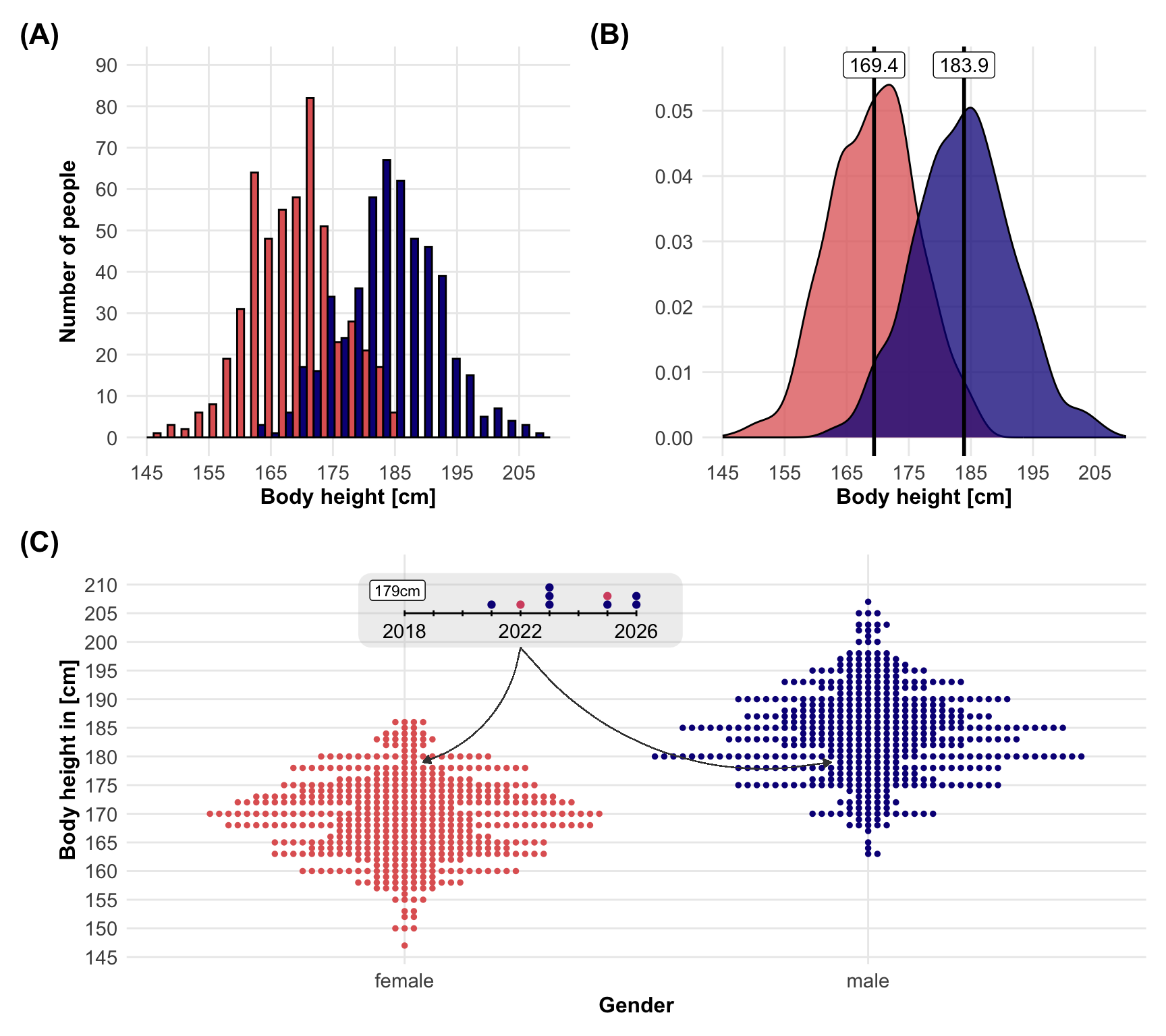
#| fig-cap: "Information regarding the internal data integration of the individual reported height. No measuring tape was used to determine body size. The different heights for both genders are shown.  **(A)** The top left shows body size as a histogram for both genders, with a bin size of 5 cm.  **(B)** The top right shows density plots of body height for both genders. The line indicates the mean. There is a shift to the right for both genders.  **(C)** The lower figure shows a beeswarm plot divided by gender. Men with a body height of 179 cm are especially rare. Men of this height have only started to appear in recent years."

mean_tbl <- gummy_student_tbl |>
  group_by(gender) |>
  summarise(mean = round(mean(height, na.rm = TRUE), 1)) |>
  na.omit()

p1 <- gummy_student_tbl |>
ggplot(aes(x = height, fill = gender)) +
  theme_book() +
  geom_histogram(position = "dodge", color = "black") +
  scale_fill_viridis(option = "plasma", discrete = TRUE, end = 0.6, direction = -1) +
  labs(x = "Body height [cm]", y = "Number of people", fill = "Geschlecht") +
  scale_x_continuous(breaks = seq(145, 215, by = 10), limits = c(145, 210)) +
  scale_y_continuous(breaks = seq(0, 90, 10), limits = c(0, 90)) +
  theme(legend.position = "none")

p2 <- gummy_student_tbl |>
ggplot(aes(x = height, fill = gender)) +
  theme_book() +
  geom_density(alpha = 0.75) +
  labs(x = "Body height [cm]", y = "", fill = "") +
  scale_x_continuous(breaks = seq(145, 215, by = 10), limits = c(145, 210)) +
  scale_y_continuous(breaks = seq(0, 0.055, 0.01), limits = c(0, 0.057)) +
  scale_fill_viridis(option = "plasma", discrete = TRUE, end = 0.6, direction = -1) +
  geom_vline(xintercept = mean_tbl$mean, color = "black",
             size = 1) +
  annotate("label", x = mean_tbl$mean, y = 0.057, label = mean_tbl$mean) +
  theme(legend.position = "none") #c(0.85, 0.8))

p3 <-
  gummy_student_tbl |>
  na.omit() |>
  ggplot(aes(x = gender, y = height, color = gender)) +
  theme_book() +
  geom_beeswarm(size = 1) +
  scale_color_viridis(option = "plasma", discrete = TRUE, end = 0.6, direction = -1) +
  labs(x = "Gender", y = "Body height in [cm]") +
  theme(legend.position = "none") +
  scale_y_continuous(breaks = seq(140, 214, 5)) +
  geom_shape(data = tibble(x = c(0.9, 1.6, 1.6, 0.9),
                           y = c(199, 199, 212, 212)), alpha = 0.25,
             aes(x, y), radius = unit(0.25, 'cm'), fill = "gray", inherit.aes = FALSE) +
  annotate("segment", x = 1, y = 205, xend = 1.5, yend = 205) +
  annotate("segment", x = seq(1, 1.5, 0.0625), xend = seq(1, 1.5, 0.0625), y = 204.5, yend = 205.5) +
  annotate("text", x = c(1, 1.25, 1.5), y = 202, label = c("2018", "2022", "2026")) +
  annotate("point", x = c(3*0.0625+1, 5*0.0625+1, 7*0.0625+1, 8*0.0625+1), y = c(206.5),
           color = "#0D0887FF") +
  annotate("point", x = c(5*0.0625+1, 8*0.0625+1), y = c(208), color = "#0D0887FF")  +
  annotate("point", x = c(5*0.0625+1), y = c(209.5), color = "#0D0887FF") +
  annotate("point", x = c(4*0.0625+1), y = c(206.5),
           color = "#D5536FFF") +
  annotate("point", x = c(7*0.0625+1), y = c(208), color = "#D5536FFF")  +
  geom_curve(aes(x = 1.25, y = 199, xend = 1.92, yend = 179),
             arrow = arrow(length = unit(0.02, "npc"), type = "closed"),
             curvature = 0.3, color = "gray25", linewidth = 0.25) +
  geom_curve(aes(x = 1.25, y = 199, xend = 1.04, yend = 179),
             arrow = arrow(length = unit(0.02, "npc"), type = "closed"),
             curvature = -0.3, color = "gray25", linewidth = 0.25) +
  annotate("label", hjust = "left", x = 0.925, y = 209, label = "179cm", size = 3)

(p1 | p2) /
  p3 +
  plot_annotation(tag_levels = 'A') +
  plot_annotation(tag_levels = 'A', tag_prefix = '(', tag_suffix = ')') &
  theme(plot.tag = element_text(size = 16, face = "bold"))

```

### Most liked gummy bear taste

```{r}
#| echo: false
#| message: false
#| warning: false
#| label: fig-chap-interlude-I-hist-taste
#| fig-align: center
#| fig-height: 4
#| fig-width: 9.5
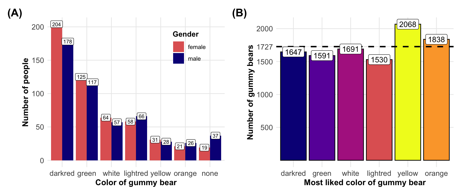
#| fig-cap: "Does Haribo know the common people's preferences for gummy bears? Yes, but does Haribo care? Have they changed the production cycle to prioritise the most popular bears? **(A)** The number of people split by gender who liked which taste the most. **(B)** The number of gummy bears in all opened bags, split by colour. In the case of a uniform distribution, the same number of colours are produced, and each colour has an equal chance of being chosen. Therefore, the number of colours should be the dotted line."

gummy_taste_tbl <- gummy_student_tbl |>
  mutate(most_liked = factor(most_liked,
                             levels = c("darkred", "green", "white", "lightred",
                                        "yellow", "orange", "none"))) |>
  na.omit()


p1 <- ggplot(data = gummy_taste_tbl, aes(x = most_liked, fill = gender)) +
  theme_book() +
  geom_bar(position = "dodge") +
  #scale_x_continuous(breaks = seq(5, 15, by = 1), limits = c(5, 15)) +
  labs(x = "Color of gummy bear", y = "Number of people", fill = "Gender") +
  theme(legend.position = c(0.8, 0.8)) +
  geom_label(stat='count', aes(label=..count.., group = gender),
             size = 2.75, fill = "white", position = position_dodge(0.9)) +
  scale_fill_viridis(option = "plasma", discrete = TRUE, end = 0.6, direction = -1)


gummy_color_tbl <- read_excel("data/gummibears.xlsx") |>
  select(darkred:white) |>
  gather(color, count)

count_bag_tbl <- rep(gummy_color_tbl$color, gummy_color_tbl$count) |>
  as_tibble() |>
  mutate(value = factor(value,
                        levels = c("darkred", "green", "white", "lightred",
                                   "yellow", "orange", "none")))

p2 <- ggplot(count_bag_tbl, aes(value)) +
  theme_book() +
  geom_bar(position = "dodge", color = "black",
           fill = c("#0D0887FF", "#6A00A8FF", "#B12A90FF", "#E16462FF" ,"#F0F921FF", "#FCA636FF")) +
  labs(x = "Most liked color of gummy bear", y = "Number of gummy bears")  +
  geom_hline(yintercept = floor(nrow(count_bag_tbl)/6),
             linetype = 2, size = 1) +
  geom_label(stat='count', aes(label=..count..), size = 4) +
  scale_y_continuous(breaks = c(500, 1000, 1500, floor(nrow(count_bag_tbl)/6), 2000))

p1 + p2 +
  plot_layout(ncol = 2) +
  plot_annotation(tag_levels = 'A') +
  plot_annotation(tag_levels = 'A', tag_prefix = '(', tag_suffix = ')') &
  theme(plot.tag = element_text(size = 16, face = "bold"))
```

```{r}
#| echo: false
#| message: false
#| warning: false
#| label: fig-chap-interlude-I-mosaic-taste
#| fig-align: center
#| fig-height: 5
#| fig-width: 9
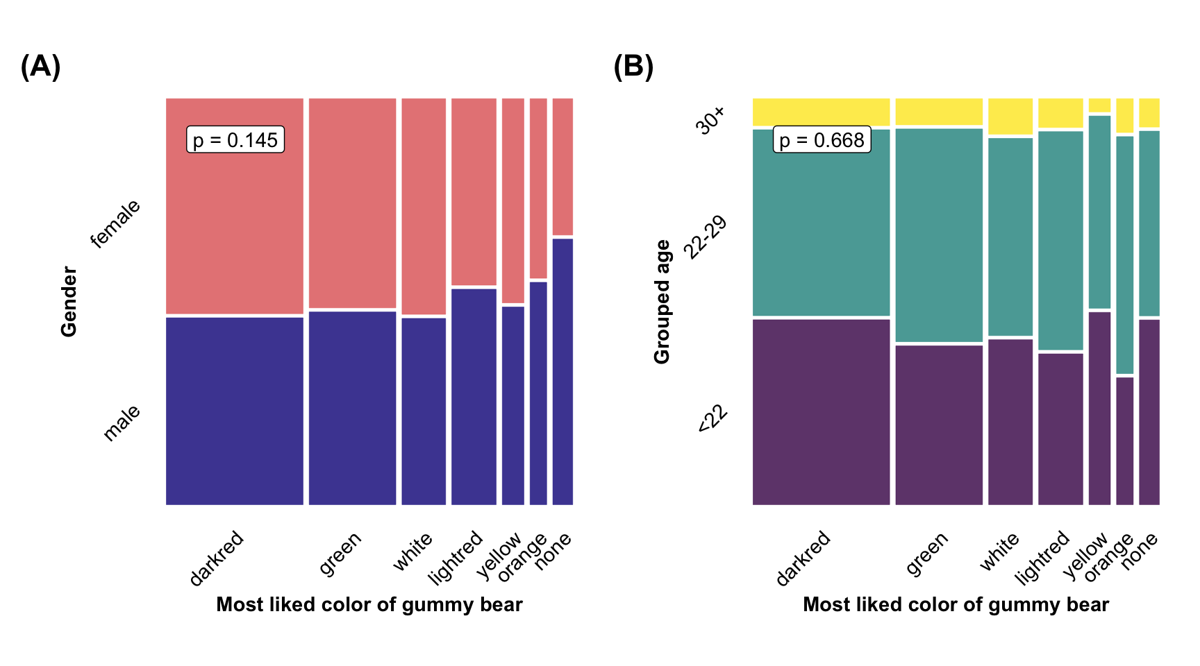
#| fig-cap: "Visualisation of the most liked colour taste of the gummy bears by a mosaic plot. **(A)** The plot on the left shows the separation of taste preferences by gender. The global chi-square test is not significant; there are no different taste preferences between the two genders. **(B)** The right plot shows the separation of the gummy bear taste preferences by three different age groups. The global chi-square test is not significant; there are no differences in taste preference between the different age groups of participants."


gummi_mosaic_tab <- gummy_student_tbl |>
  select(gender, age_grp, most_liked) |>
  mutate(most_liked = factor(most_liked,
                             levels = c("darkred", "green", "white", "lightred",
                                        "yellow", "orange", "none"))) |>
  mutate(gender = fct_rev(gender))

p_gender <- gummi_mosaic_tab |>
  na.omit() |>
  tabyl(gender, most_liked) |>
  janitor::chisq.test() |>
  broom::tidy() |>
  pull(p.value) |>
  scales::pvalue()

p_age <- gummi_mosaic_tab |>
  na.omit() |>
  tabyl(age_grp, most_liked) |>
  janitor::chisq.test() |>
  broom::tidy() |>
  pull(p.value) |>
  scales::pvalue()

p1 <- gummi_mosaic_tab |>
  select(gender, most_liked) |>
  ftable() |>
  as.data.frame() |>
  ggplot(aes(x = product(gender, most_liked), weight = Freq, fill = gender)) +
  theme_book() +
  geom_mosaic() +
  theme_mosaic(rot_labels = 45) +
  scale_fill_viridis(option = "plasma", discrete = TRUE, end = 0.6, direction = 1) +
  theme(legend.position = "none") +
  labs(x = "Most liked color of gummy bear", y = "Gender") +
  annotate("label", x = 0.05, y = 0.9, label = str_c("p = ", p_gender), hjust = "left")

p2 <- gummi_mosaic_tab |>
  select(age_grp, most_liked) |>
  ftable() |>
  as.data.frame() |>
  ggplot(aes(x = product(age_grp, most_liked), weight = Freq, fill = age_grp)) +
  theme_book() +
  geom_mosaic() +
  theme_mosaic(rot_labels = 45) +
  scale_fill_viridis_d() +
  theme(legend.position = "none") +
  labs(x = "Most liked color of gummy bear", y = "Grouped age") +
  annotate("label", x = 0.05, y = 0.9, label = str_c("p = ", p_age), hjust = "left")

p1 + p2 +
  plot_layout(ncol = 2) +
  plot_annotation(tag_levels = 'A') +
  plot_annotation(tag_levels = 'A', tag_prefix = '(', tag_suffix = ')') &
  theme(plot.tag = element_text(size = 16, face = "bold"))
```

### The gummy bear lottery

$$
f(y \mid\mu,\sigma^2)=\cfrac{1}{\sqrt{2\pi\sigma^2}} e^{-\cfrac{(y-\mu)^2}{2\sigma^2}}\quad -\infty<y<\infty
$$

$$
\begin{align*}
Pr(c=1|b) &= \tfrac{1}{6}^{b-1}  \mbox{\; for\;} b \in \{1,..., 15\} \\
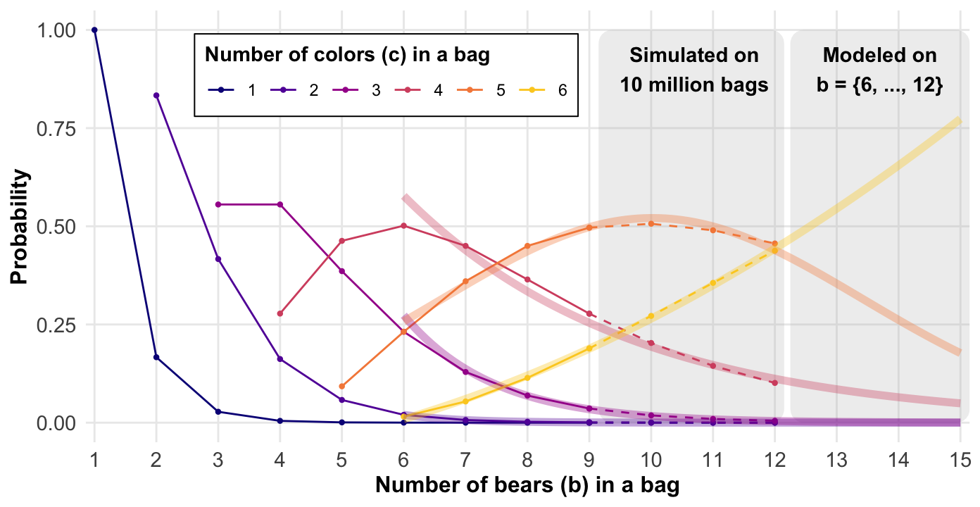
Pr(c=2|b) &= 14.53 \cdot \tfrac{1}{3}^{b} \mbox{\; for\;} b \in \{6,..., 15\}\\
Pr(c=3|b) &= 17.5 \cdot \tfrac{1}{2}^{b} \mbox{\; for\;} b \in \{6,..., 15\}\\
Pr(c=4|b) &= 2.98 \cdot 0.7607^b \mbox{\; for\;} b \in \{6,..., 15\}\\
Pr(c=5|b) &= 0.521 \cdot e^{-\tfrac{(b-10.02)^2}{(2\cdot3.39^2)}} \mbox{\; for\;} b \in \{6,..., 15\}\\
Pr(c=6|b) &= 0.00419 \cdot b^2-0.00303 \cdot b-0.12376 \mbox{\; for\;} b \in \{6,..., 15\}\\
\end{align*}
$$

```{r}
#| echo: false
#| message: false
#| warning: false
#| label: fig-chap-interlude-I-grid
#| fig-align: center
#| fig-height: 3.75
#| fig-width: 7.25
#| fig-cap: "Probability of observation of the number of colours given the number of bears in a bag. The first nine bag sizes could be solved using combination and by counting the number of colours in a bag of a given size. However, the results for 10 to 12 bears in a bag had to be obtained by simulation and drawing 10 million bags due to performance issues. Gemini 3.5 (Flash-Lite), Excel and R with `{nlme}` were used to optimise the modelling and generation of the shaded graphs."

grid_table_tbl <- read_excel("data/grid_table.xlsx") |>
  pivot_longer(cols = b01:b12,
               values_to = "percent",
               names_to = "bears") |>
  mutate(c = as_factor(c),
         bears = as.numeric(as.factor(bears)))

filter(grid_table_tbl, bears %in% 1:9) |>
  ggplot(aes(x = bears, y = percent, color = c)) +
  theme_book() +
  geom_shape(data = tibble(bears = c(9.15, 12.15, 12.15, 9.15),
                           percent = c(0, 0, 1, 1),
                           c = NA),
             aes(bears, percent), radius = unit(0.25, 'cm'), fill = "gray",
             show.legend = FALSE, alpha = 0.25, inherit.aes = FALSE) +
  annotate("text", x = 10.7, y = 0.9, label = "Simulated on\n10 million bags",
           fontface = 2) +
  geom_shape(data = tibble(bears = c(12.25, 15.15, 15.15, 12.25),
                           percent = c(0, 0, 1, 1),
                           c = NA),
             aes(bears, percent), radius = unit(0.25, 'cm'), fill = "gray",
             show.legend = FALSE, alpha = 0.25, inherit.aes = FALSE) +
  annotate("text", x = 13.7, y = 0.9, label = "Modeled on\nb = {6, ..., 12}",
           fontface = 2) +
  geom_line() +
  geom_line(data = filter(grid_table_tbl, bears %in% 9:12),
            linetype = 2, show.legend = FALSE) +
  geom_point2() +
  geom_point2(data = filter(grid_table_tbl, bears %in% 9:12),
              show.legend = FALSE) +
  scale_x_continuous(breaks = 1:15, expand = expansion(mult = c(0.01, 0))) +
  labs(color = "Number of colors (c) in a bag", x = "Number of bears (b) in a bag",
       y = "Probability") +
  scale_color_viridis(option = "plasma", discrete = TRUE, end = 0.9) +
  geom_function(fun = \(x) 14.53 * 1/3^x, xlim = c(6, 15), color = "#6300A7FF", size = 2, alpha = 0.35) +
  geom_function(fun = \(x) 17.5 * 1/2^x, xlim = c(6, 15), color = "#A51F99FF", size = 2, alpha = 0.35) +
  geom_function(fun = \(x) 2.98 * 0.7607^x, xlim = c(6, 15), color = "#D5536FFF", size = 2, alpha = 0.35) +
  geom_function(fun = \(x) 0.521 * exp(-((x-10.02)^2/(2*3.39^2))), xlim = c(6, 15),
                color = "#F58A47FF", size = 2, alpha = 0.35) +
  geom_function(fun = \(x) 0.00419*x^2-0.00303*x-0.12376, xlim = c(6, 15),
                color = "#FCCE25FF", size = 2, alpha = 0.35) +
  guides(color = guide_legend(nrow = 1, byrow = TRUE)) +
  theme(legend.position = c(0.34, 0.85),
        legend.box.background = element_rect(color = "black"))
```

```{r}
#| echo: false
#| message: false
#| warning: false
#| label: fig-chap-interlude-I-obs-exp
#| fig-align: center
#| fig-height: 3.25
#| fig-width: 7
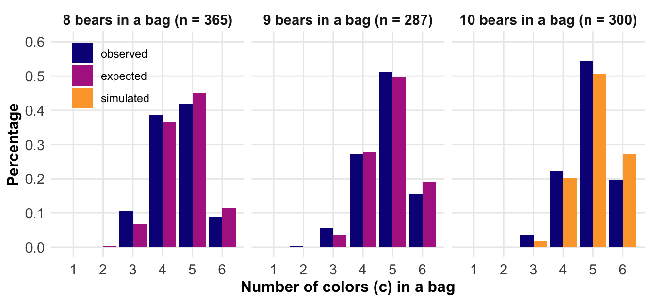
#| fig-cap: "Percentage of observed numbers of colours in a bag given different bag sizes. On the left are the observed and expected percentages of eight bears in a bag. In the middle, the observed and expected numbers of colours in a bag containing nine bears. On the right, the observed and simulated percentages for a bag containing 10 bears. The simulation was necessary because calculating the expected values would take too long."

bear_8_vec <- gummy_count_tbl |>
  filter(bear_exp == 8) |>
  tabyl(color_exp) |>
  pull("percent")

bear_9_vec <- gummy_count_tbl |>
  filter(bear_exp == 9) |>
  tabyl(color_exp) |>
  pull("percent")

bear_10_vec <- gummy_count_tbl |>
  filter(bear_exp == 10) |>
  tabyl(color_exp) |>
  pull("percent")

bear_8_n <- gummy_count_tbl |>
  filter(bear_exp == 8) |>
  tabyl(color_exp) |>
  pull("n") |>
  sum()

bear_9_n <- gummy_count_tbl |>
  filter(bear_exp == 9) |>
  tabyl(color_exp) |>
  pull("n") |>
  sum()

bear_10_n <- gummy_count_tbl |>
  filter(bear_exp == 10) |>
  tabyl(color_exp) |>
  pull("n") |>
  sum()

rbind(tibble(type = gl(2, 6, labels = c("observed", "expected")),
             color = rep(1:6, 2),
             percent = c(c(0, 0, bear_8_vec),
                         0, 0.002268376, 0.069015775, 0.364583333, 0.450102881, 0.114026063),
             bears = str_c("8 bears in a bag (n = ", bear_8_n, ")")),
      tibble(type = gl(2, 6, labels = c("observed", "expected")),
             color = rep(1:6, 2),
             percent = c(c(0, bear_9_vec),
                         0, 0.000759102, 0.036020138, 0.277563443, 0.496613512, 0.18904321),
             bears = str_c("9 bears in a bag (n = ", bear_9_n, ")")),
      tibble(type = gl(2, 6, labels = c("observed", "simulated")),
             color = rep(1:6, 2),
             percent = c(c(0, 0, bear_10_vec),
                         0, 0.0002601, 0.0185012, 0.2029175, 0.5064902, 0.271831),
             bears = str_c("10 bears in a bag (n = ", bear_10_n, ")"))
)  |>
  mutate(bears = as_factor(bears)) |>
  ggplot(aes(x = color, y = percent, fill = type)) +
  theme_book() +
  geom_bar(stat = "identity", position = position_dodge()) +
  scale_x_continuous(breaks = 1:6) +
  scale_y_continuous(limits = c(0, 0.6), breaks = seq(0, 0.6, 0.1)) +
  scale_fill_viridis(option = "plasma", discrete = TRUE, end = 0.8) +
  labs(fill = "", y = "Percentage", x = "Number of colors (c) in a bag") +
  theme(legend.position = c(0.1, 0.85)) +
  facet_wrap(~bears)

```

```{r}
#| echo: false
#| message: false
#| warning: false
#| label: tbl-gummy-prob-table
#| tbl-cap: "The final table to judge the probability of observing c colours in a bag containing between 6 and 15 gummy bears. It can be assumed that bags containing fewer than six bears will never be produced. With seven gummy bears in a bag, the likelihood of finding only one colour is approximately 1 in 46,000."

read_excel("data/grid_table.xlsx") |>
  select(c, b06:b15) |>
  mutate_all(round, 4) |>
  mutate(across(2:11, scales::percent)) |>
  set_names(c("Colors", 6:15)) |>
  kable(align = "c", "pipe") |>
  add_header_above(c(" " = 1, "Combined" = 4, "Simulated" = 3, "Modeled" = 3)) |>
  add_header_above(c(" " = 1, "Bears " = 10))
```

With seven bears in a bag, I would like to have opened roughly 46,656 bags to find a bag with only one color of bear. With eight bears in a bag, it would be an astonishing 279,936 bags. Currently, I have an average of `r round(mean(count_tbl$n[-c(1:3)]))` bags counted per year among my lectures in the last five years. I still believe that the number of bears in a bag will remain stable at eight in the coming years. In this case, on average, I would need `r round(279936/round(mean(count_tbl$n[-c(1:3)])))` years before I would find one of a different colour. Even if Haribo reduces the number of bears in a bag to seven, it would still take me `r round(46656/round(mean(count_tbl$n[-c(1:3)])))` years to reach my goal. Therefore, in answer to my initial research question, I realise that I have little chance of achieving my goal in my lifetime. But this will not stop me — maybe I'll get lucky and the next bag will contain only one colour. The only assumption I have to make is that Haribo does not rig the filling process of the bags and removes any coloured bags that appear. It would be a bittersweet symphony.

The @tbl-probability-comparison shows a collection of odds for rare events that are not taken too seriously. Therefore, finding a one-coloured bag containing eight bears would be as unlikely as being bitten by a snake or hit by a comet in a lifetime. Neither event is more preferable than a bag of coloured bears. The table should not be taken too seriously. I gathered the information from a quick web search and did not consult any scientific references.

| Event                                        | Odds           |
|:---------------------------------------------|:---------------|
| Odds to win Lotto 6 out of 49                | $1:15,537,573$ |
| Annual risk of being killed in a plane crash | $1:11,000,000$ |
| Lifetime odds to be hit by a comet           | $1:1,600,000$  |
| **Bag of 8 bears with one color**            | $\mathbf{1:279,936}$    |
| Bitten by a snake in everyday life           | $1:40,000$     |
| Struck by lightning in a lifetime            | $1:15,300$     |
| Lifetime odds of dying in a car crash        | $1:100$        |
| Getting cancer in a lifetime                 | $1:5$          |
| Odds to be eaten by a polar bear             | $>0$          |

: A not-so-serious table of rare events and their odds of happening. {#tbl-probability-comparison}

Well, dear reader, we’ve come to the end of this section. For me, the journey continues—I’ll keep tearing open packets and counting the bears. But you’re probably eager to learn more about the statistics by now. That’s what we’ll cover in the next few chapters.

## Alternatives

Further tutorials and R packages on XXX

## Glossary

term

: what does it mean.

## The meaning of "Models of Reality" in this chapter.

- itemize with max. 5-6 words

## Summary

## References {.unnumbered}