5 Eating habits of fleas
Last modified on 06. June 2026 at 20:42:16
“A quote.” — Dan Meyer
5.1 General background
What is a data grid?
5.2 Theoretical background
5.3 R packages used
R Code [show / hide]
pacman::p_load(tidyverse, conflicted)5.4 Data
Small data and grid
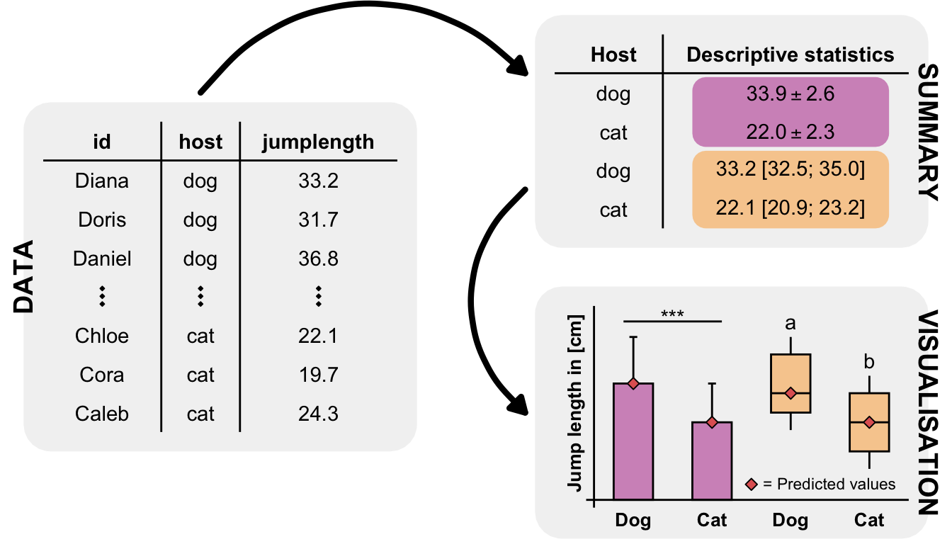
5.4.1 Fleas with feeding habits
C. felis felis jump was \(19.9 \pm 9.1cm\) with a range from \(2\) to \(48cm\)
C. canis jump was longer \(30.4 \pm 9.1cm\) with a range from \(3\) to \(50cm\)
The jump length of P. irritans has to be derived from the work of Cadiergues et al. (2000)2 because no mean or standard deviation for the human flea was available.
Miarinjara (2025) et al.3 demonstrate the impact of sheep’s blood on the jumping ability of human fleas.
R Code [show / hide]
jump_flea_grid <- expand_grid(feeding = c("sugar water", "human blood")) |>
  mutate(mean = c(19.9, 30.4),
         sd = c(9.1))
R Code [show / hide]
jump_flea_tbl <- jump_flea_grid |>
  rowwise() |>
  mutate(jumplength = lst(rnorm(7, mean, sd))) |>
  unnest(cols = jumplength) |>
  mutate(feeding = as_factor(feeding))
R Code [show / hide]
jump_flea_tbl |>
  group_by(feeding) |>
  summarise(mean(jumplength),
            sd(jumplength)) |>
  mutate_if(is.numeric, round, 2)
# A tibble: 2 × 3
feeding `mean(jumplength)` `sd(jumplength)`
<fct> <dbl> <dbl>
1 sugar water 21.2 7.3
2 human blood 33.0 6.57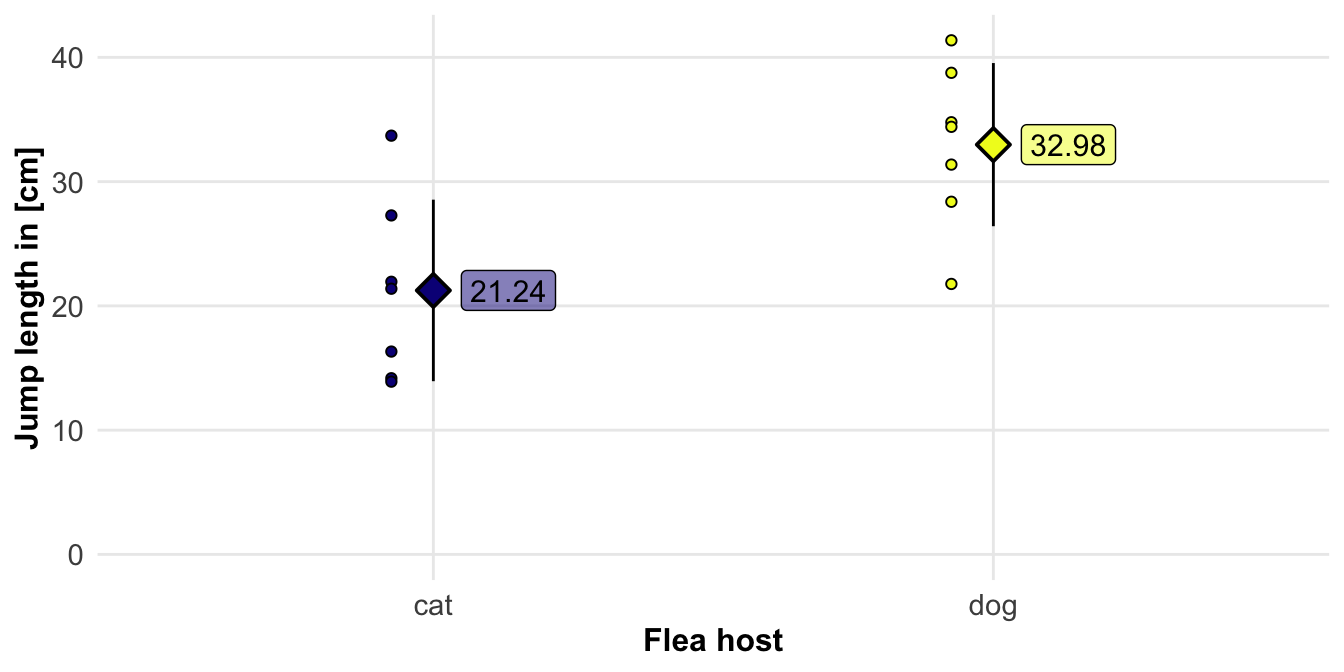
R Code [show / hide]
jump_animals_grid <- expand_grid(feeding = c("sugar water", "tomato ketchup", "fake blood", "human blood")) |>
  mutate(mean = c(19.9, 35.2, 15.2, 30.4),
         sd = c(9.1, 10.3, 4.6, 9.1))
R Code [show / hide]
jump_animals_tbl <- jump_animals_grid |>
  rowwise() |>
  mutate(jumplength = lst(rnorm(7, mean, sd))) |>
  unnest(cols = jumplength) |>
  mutate(feeding = as_factor(feeding))
R Code [show / hide]
jump_animals_tbl |>
  group_by(feeding) |>
  summarise(mean(jumplength),
            sd(jumplength)) |>
  mutate_if(is.numeric, round, 2)
# A tibble: 4 × 3
feeding `mean(jumplength)` `sd(jumplength)`
<fct> <dbl> <dbl>
1 sugar water 21.2 9.36
2 tomato ketchup 34.6 10.2
3 fake blood 13.4 2.51
4 human blood 34.0 17.4 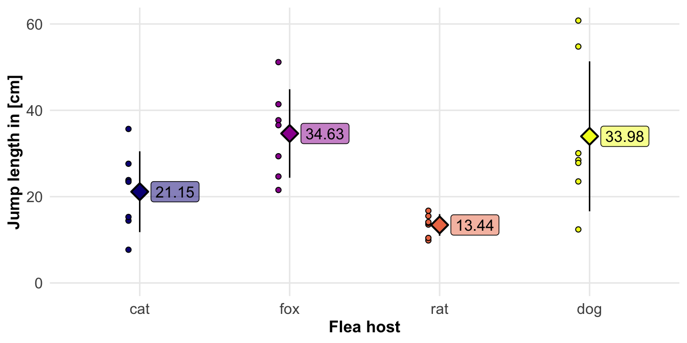
5.4.2 Fleas at stages of development
Why so complex?
R Code [show / hide]
jump_habitat_grid <- expand_grid(feeding = 1:3, stage = 1:2) |>
  mutate(mean_feeding = c(19.9, 19.9, 30.4, 30.4, 15.2, 15.2),
         mean_stage = c(5, 0, 5, 0, 5, -5),
         mean = mean_feeding + mean_stage,
         sd = c(9.1, 9.1, 9.1, 9.1, 4.6, 4.6))
jump_habitat_grid
# A tibble: 6 × 6
feeding stage mean_feeding mean_stage mean sd
<int> <int> <dbl> <dbl> <dbl> <dbl>
1 1 1 19.9 5 24.9 9.1
2 1 2 19.9 0 19.9 9.1
3 2 1 30.4 5 35.4 9.1
4 2 2 30.4 0 30.4 9.1
5 3 1 15.2 5 20.2 4.6
6 3 2 15.2 -5 10.2 4.6R Code [show / hide]
jump_habitat_raw_tbl <- jump_habitat_grid |>
  rowwise() |>
  mutate(jumplength = lst(rnorm(7, mean, sd))) |>
  unnest(cols = jumplength)
R Code [show / hide]
jump_habitat_tbl <- jump_habitat_raw_tbl |>
  select(feeding, stage, jumplength) |>
  mutate(feeding = factor(feeding, labels = c("sugar water", "tomato ketchup", "human blood")),
         stage = factor(stage, labels = c("juvenile", "adult"))) |>
  mutate_if(is.numeric, round, 2)
R Code [show / hide]
jump_habitat_tbl |>
  group_by(feeding, stage) |>
  summarise(mean(jumplength),
            sd(jumplength)) |>
  mutate_if(is.numeric, round, 2)
# A tibble: 6 × 4
# Groups: feeding [3]
feeding stage `mean(jumplength)` `sd(jumplength)`
<fct> <fct> <dbl> <dbl>
1 sugar water juvenile 25.1 13.8
2 sugar water adult 14.9 11.4
3 tomato ketchup juvenile 29.9 6.32
4 tomato ketchup adult 27.3 9.26
5 human blood juvenile 22.0 3.65
6 human blood adult 10.1 4.6 
5.4.3 Measurements on animal fleas
- Jump length in [cm] called
jump_length - Number of hairs on each leg called
count_leg_leftandcount_leg_right - Ratings of each flea, as listed in the catalog of the Fédération Internationale de la Beauté des Puces (FIBP) called
ratingon a Likert scale from 1 to 5, with 5 being the strongest expression. - The infection status with the flea cold is called
infected, with a value of 0/1 for no/yes.
R Code [show / hide]
tibble(jumplength = rnorm(7, 5, 1),
       counthairleg_left = rpois(7, 4),
       counthairleg_right = rpois(7, 4),
       counthairleg = (counthairleg_left + counthairleg_right)/2,
       rating = sample(1:5, 7, replace = TRUE, prob = c(0.1, 0.2, 0.4, 0.2, 0.1)),
       infectd = rbinom(7, prob = 0.5, size = 1))
# A tibble: 7 × 6
jumplength counthairleg_left counthairleg_right counthairleg rating infectd
<dbl> <int> <int> <dbl> <int> <int>
1 5.02 3 5 4 2 0
2 4.73 6 4 5 3 0
3 5.91 4 5 4.5 3 0
4 3.38 6 3 4.5 2 1
5 3.10 3 4 3.5 5 0
6 7.02 4 3 3.5 1 1
7 3.95 4 3 3.5 1 05.5 Data availability
The data is available as txt-Files under https://github.com/jkruppa/biodatascience.
5.6 Alternatives
Further tutorials and R packages on XXX
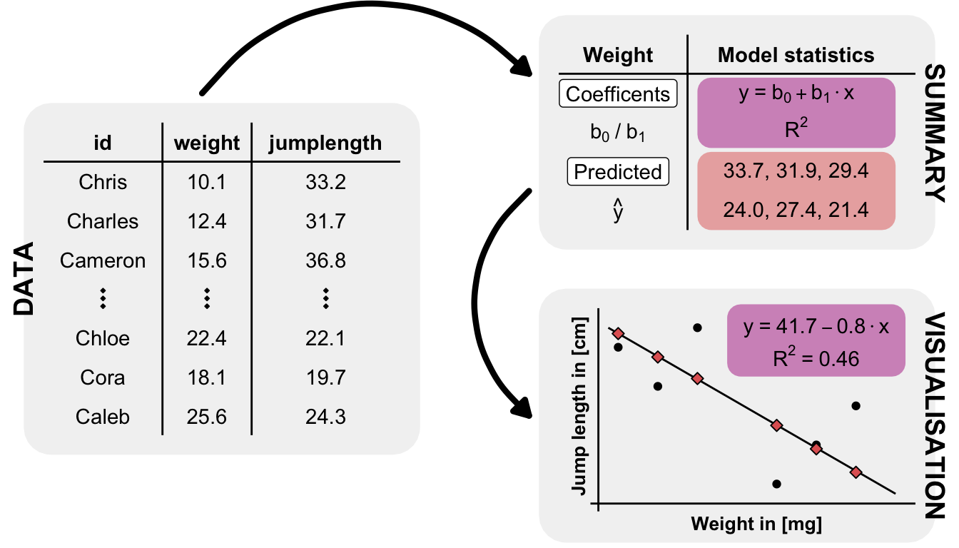
5.6.1 Why linear is a bad idea?
R Code [show / hide]
jump_flea_tbl <- tibble(feeding = rep(0:1, each = 7),
                        jump_length = 19.9 + 10.5 * feeding + rnorm(14, 0, 9.1)) |>
  mutate(feeding = factor(feeding, labels = c("cat", "dog")))
5.6.2 Why is a tibble() bad idea?
R Code [show / hide]
jump_animals_tbl <- tibble(cat = rnorm(n = 7, mean = 19.9, sd = 9.1),
                           fox = rnorm(n = 7, mean = 35.2, sd = 10.3),
                           rat = rnorm(n = 7, mean = 15.2, sd = 4.6),
                           dog = rnorm(n = 7, mean = 30.4, sd = 9.1)) |>
  pivot_longer(cols = cat:dog, values_to = "jump_length", names_to = "feeding") |>
  mutate(feeding = as_factor(feeding))
5.7 Glossary
- term
-
what does it mean.
5.8 The meaning of “Models of Reality” in this chapter.
- itemize with max. 5-6 words
5.9 Summary
References
[1]
Wickham H, Çetinkaya-Rundel M, Grolemund G. R for Data Science: Import, Tidy, Transform, Visualize, and Model Data. " O’Reilly Media, Inc."; 2023.
[2]
Cadiergues MC, Joubert C, Franc M. A comparison of jump performances of the dog flea, ctenocephalides canis (curtis, 1826) and the cat flea, ctenocephalides felis felis (bouché, 1835). Veterinary parasitology. 2000;92(3):239-241.
[3]
Miarinjara A, Raveloson AO, Rajaonarimanana M, Ayala D, Girod R, Gillespie TR. Establishing a laboratory colony of the human flea, pulex irritans: Methods for collecting, rearing, and feeding. Parasites & Vectors. 2025;18(1):363.
[4]
Wickham H, Henry L. Purrr: Functional Programming Tools.; 2025. https://purrr.tidyverse.org/