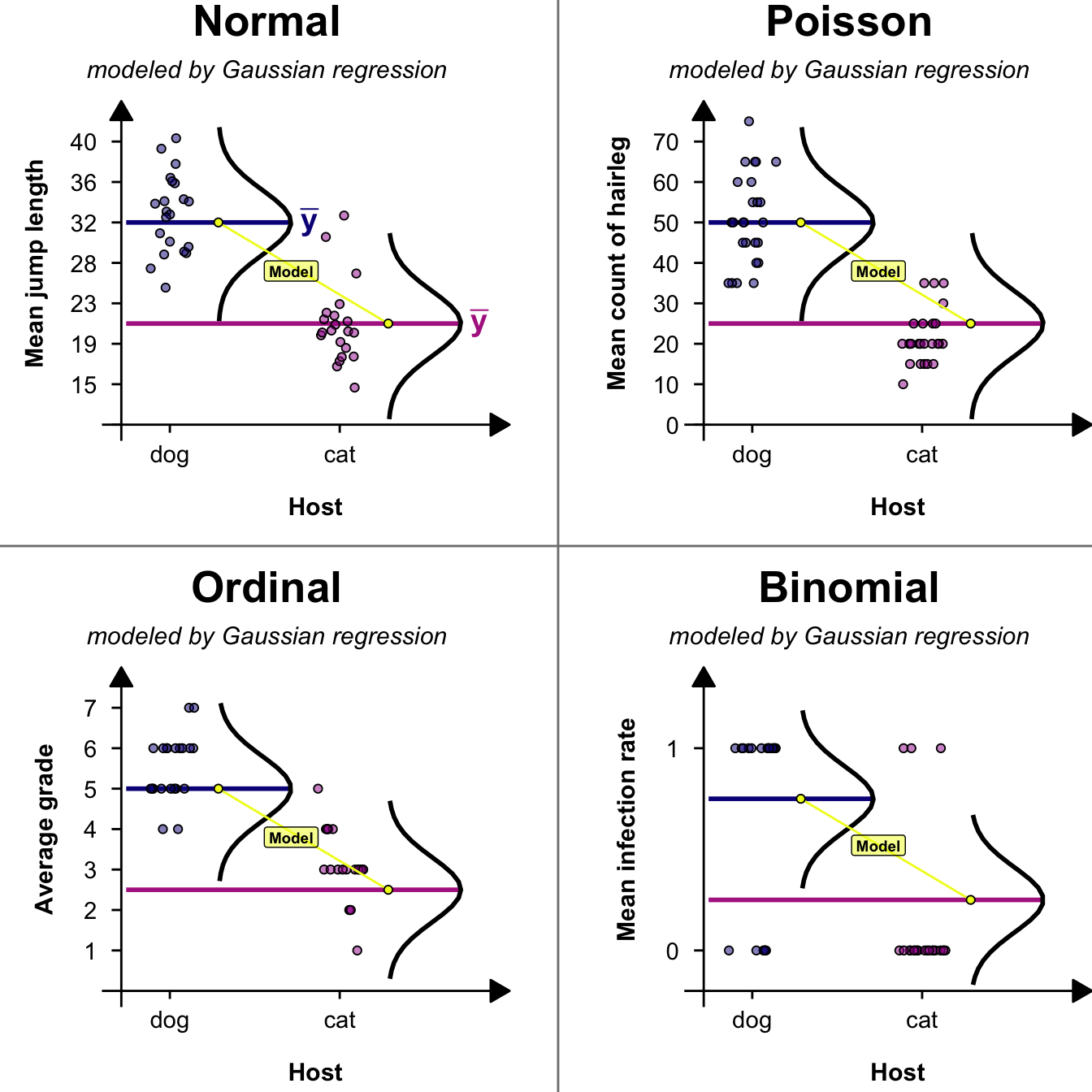
Visualisation of data

Last modified on 20. December 2025 at 20:24:43

“What problem have you solved, ever, that was worth solving where you knew all the given information in advance? No problem worth solving is like that. In the real world, you have a surplus of information and you have to filter it, or you don’t have sufficient information and you have to go find some.” — Dan Meyer in Math class needs a makeover

Here comes the preface text

Figure 1: foo

pacman::p_load(emmeans, parameters, nlme, broom)

foo <- tibble(A = rnorm(10000, 5, 4),
              B = rnorm(10000, 8, 2)) |> 
  gather()

foo |> 
  group_by(key) |> 
  summarise(mean(value), var(value), sd(value))

# A tibble: 2 × 4
  key   `mean(value)` `var(value)` `sd(value)`
  <chr>         <dbl>        <dbl>       <dbl>
1 A              4.99        16.1         4.02
2 B              8.01         4.03        2.01

sqrt((16.77840 + 3.94372)/2)    

[1] 3.21886

fit <- lm(value ~ 0+key, foo)

fit |> parameters()

Parameter | Coefficient |   SE |       95% CI | t(19998) |      p
-----------------------------------------------------------------
key [A]   |        4.99 | 0.03 | [4.92, 5.05] |   157.01 | < .001
key [B]   |        8.01 | 0.03 | [7.95, 8.07] |   252.19 | < .001

Uncertainty intervals (equal-tailed) and p-values (two-tailed) computed
  using a Wald t-distribution approximation.

fit |> glance()

# A tibble: 1 × 12
  r.squared adj.r.squared sigma statistic p.value    df  logLik     AIC     BIC
      <dbl>         <dbl> <dbl>     <dbl>   <dbl> <dbl>   <dbl>   <dbl>   <dbl>
1     0.815         0.815  3.18    44126.       0     2 -51486. 102979. 103002.
# ℹ 3 more variables: deviance <dbl>, df.residual <int>, nobs <int>

0.02012848 * sqrt(10000)

[1] 2.012848

sqrt(diag(vcov(fit)))

      keyA       keyB 
0.03175371 0.03175371 

model_parameters(fit, vcov = "HC3")

Parameter | Coefficient |   SE |       95% CI | t(19998) |      p
-----------------------------------------------------------------
key [A]   |        4.99 | 0.04 | [4.91, 5.06] |   124.10 | < .001
key [B]   |        8.01 | 0.02 | [7.97, 8.05] |   399.10 | < .001

Uncertainty intervals (equal-tailed) and p-values (two-tailed) computed
  using a Wald t-distribution approximation.

gls(value ~ 0 + key, weights = varIdent(form =  ~ 1 | key), foo) |> 
  parameters()

# Fixed Effects

Parameter | Coefficient |   SE |       95% CI | t(19998) |      p
-----------------------------------------------------------------
key [A]   |        4.99 | 0.04 | [4.91, 5.06] |   124.10 | < .001
key [B]   |        8.01 | 0.02 | [7.97, 8.05] |   399.12 | < .001

Uncertainty intervals (equal-tailed) and p-values (two-tailed) computed
  using a Wald t-distribution approximation.

emm <- emmeans(fit, "key", vcov = sandwich::vcovHAC)
summary_emm <- summary(emm)
# Calculate SD from SE and sample size (n)
summary_emm$SE * sqrt(summary_emm$df/2) 

[1] 4.015578 2.002160