```{r echo = FALSE, warning = FALSE, message=FALSE}
source("init.R")
```
# Dining habits of fleas {#sec-temp}
*Last modified on `r format(fs::file_info("chapter-13-combined-data.qmd")$modification_time, '%d. %B %Y at %H:%M:%S')`*
> *"A quote." --- Dan Meyer*
## General background
Based on standard methods in flea research and experimental entomology, as well as a similar published experiment, the following three types of food for adult cat fleas are possible, representing different nutritional conditions:
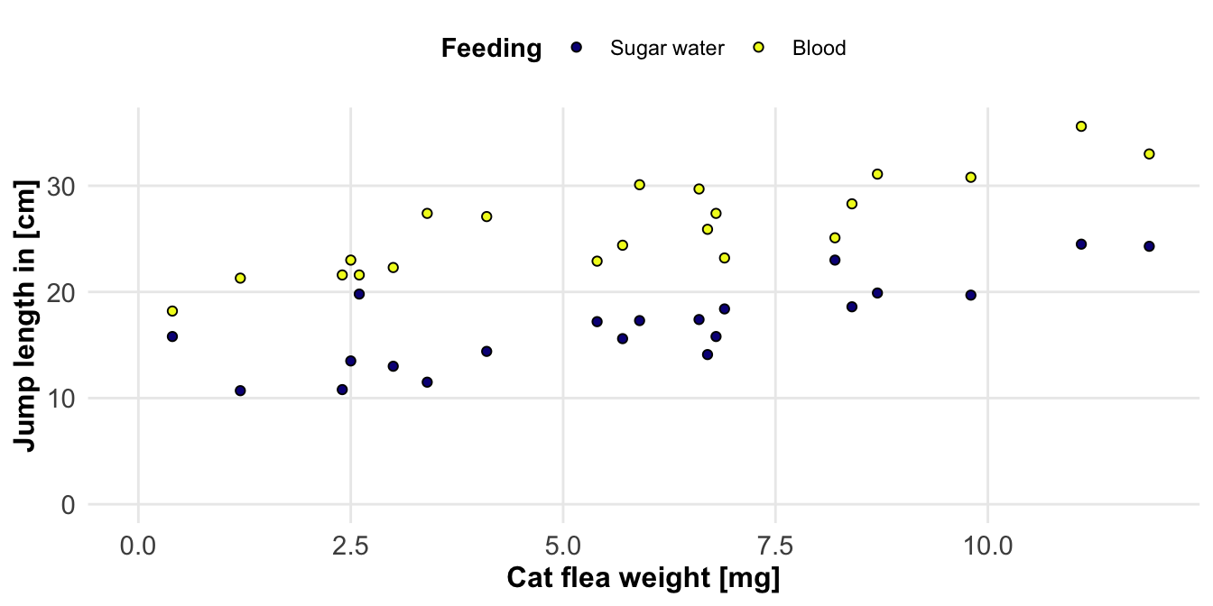
Blood: This is the natural and optimal food source for adult fleas.Often, defibrinated or anticoagulated animal blood (e.g. bovine blood, rabbit blood) is used for this purpose, which is offered in special in vitro feeding systems (e.g. through a membrane).Expectation: Fleas that are optimally nourished should show the greatest jumping distance.
Sugar water: Often serves as a ‘control feed’ or as a feed that provides energy (sugar) but lacks essential nutrients (such as proteins from blood).Expectation: Jumping distance could be reduced due to the lack of blood and thus the proteins important for reproduction, which could impair physiological fitness.
Ketchup - a nutrient-poor or unsuitable food: This option is used to simulate poor, incomplete or stressful nutritional conditions.In a similar documented experiment, ketchup (a combination of sugar, vinegar and minimal other substances, but no blood) was used as the third feed.Expectation: It can be assumed that fleas will show the shortest jumping distance under these conditions, as they lack both essential nutrients and the necessary energy.
## Theoretical background
## R packages used
## Data
### Linear
```{r}
jump_weight_feeding_tbl <- expand_grid(f = c(0, 1),
                                       x = abs(rnorm(21, 5, 4))) |>
  mutate(y = 10 + 1.2 * x + 10 * f + rnorm(42, 0, 2),
         f = factor(f, labels = c("sugar_water", "blood")))  |>
  mutate_if(is.numeric, round, 1) |>
  rename(weight = x, jumplength = y, feeding = f)
```
```{r}
#| echo: false
#| message: false
#| warning: false
#| label: fig-chap-11-cov-02
#| fig-align: center
#| fig-height: 3.5
#| fig-width: 7
#| fig-cap: "foo **(A)** foo **(B)** foo"
jump_weight_feeding_tbl |>
ggplot(aes(x = weight, y = jumplength, fill = feeding)) +
theme_book() +
geom_point(shape = 21) +
labs(x = "Cat flea weight [mg]", y = "Jump length in [cm]",
fill = "Feeding") +
scale_fill_viridis(discrete = TRUE, option = "plasma",
labels = c("Sugar water", "Blood")) +
coord_cartesian(xlim = c(0, NA), ylim = c(0, NA))
```
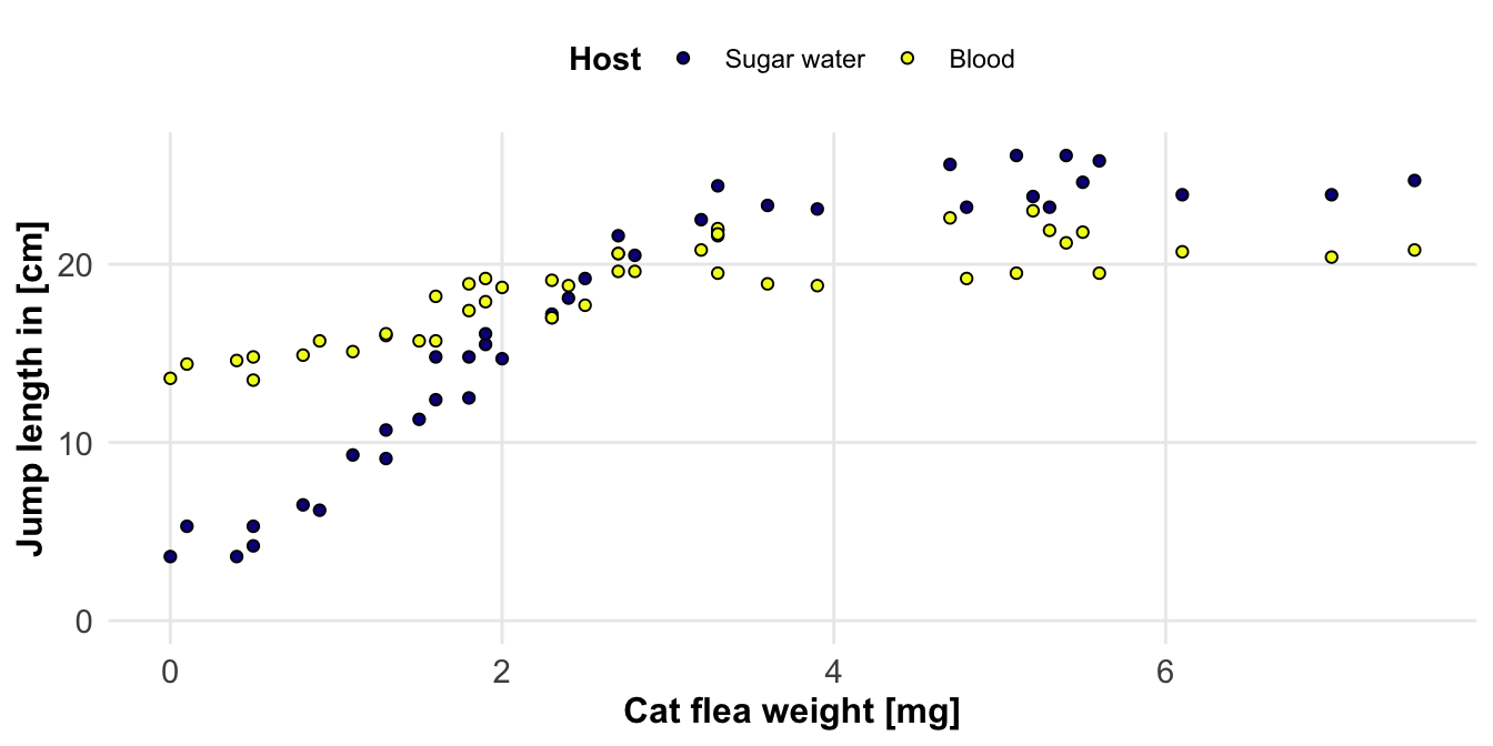
### Non linear
```{r}
jump_weight_non_linear_tbl <- expand_grid(f = c(0, 1),
                                          x = abs(rnorm(42, 2.5, 2.5))) |>
  mutate(y = 25 - 4*f - 21 * exp(-0.2 * x^2 - 1.1 * f) + rnorm(84, 0, 1),
         f = factor(f, labels = c("sugar_water", "blood")))  |>
  mutate_if(is.numeric, round, 1) |>
  rename(weight = x, jumplength = y, feeding = f)
```
```{r}
#| echo: false
#| message: false
#| warning: false
#| label: fig-chap-11-cov-05
#| fig-align: center
#| fig-height: 3.5
#| fig-width: 7
#| fig-cap: "foo **(A)** foo **(B)** foo"
jump_weight_non_linear_tbl |>
ggplot(aes(x = weight, y = jumplength, fill = feeding)) +
theme_book() +
geom_point(shape = 21) +
labs(x = "Cat flea weight [mg]", y = "Jump length in [cm]",
fill = "Host") +
scale_fill_viridis(discrete = TRUE, option = "plasma",
labels = c("Sugar water", "Blood")) +
coord_cartesian(xlim = c(0, NA), ylim = c(0, NA))
```
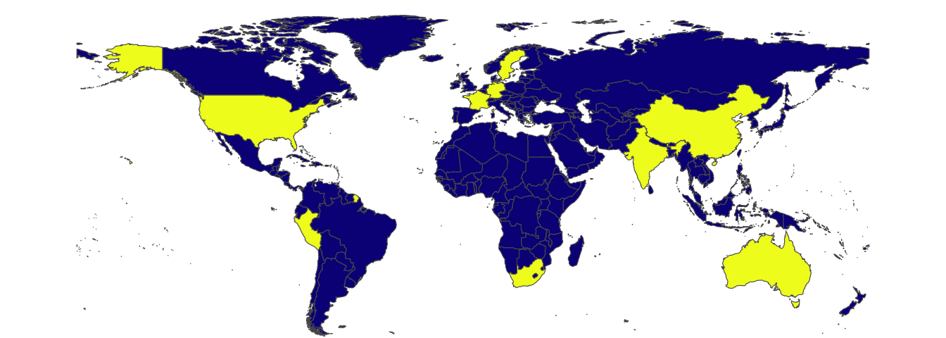
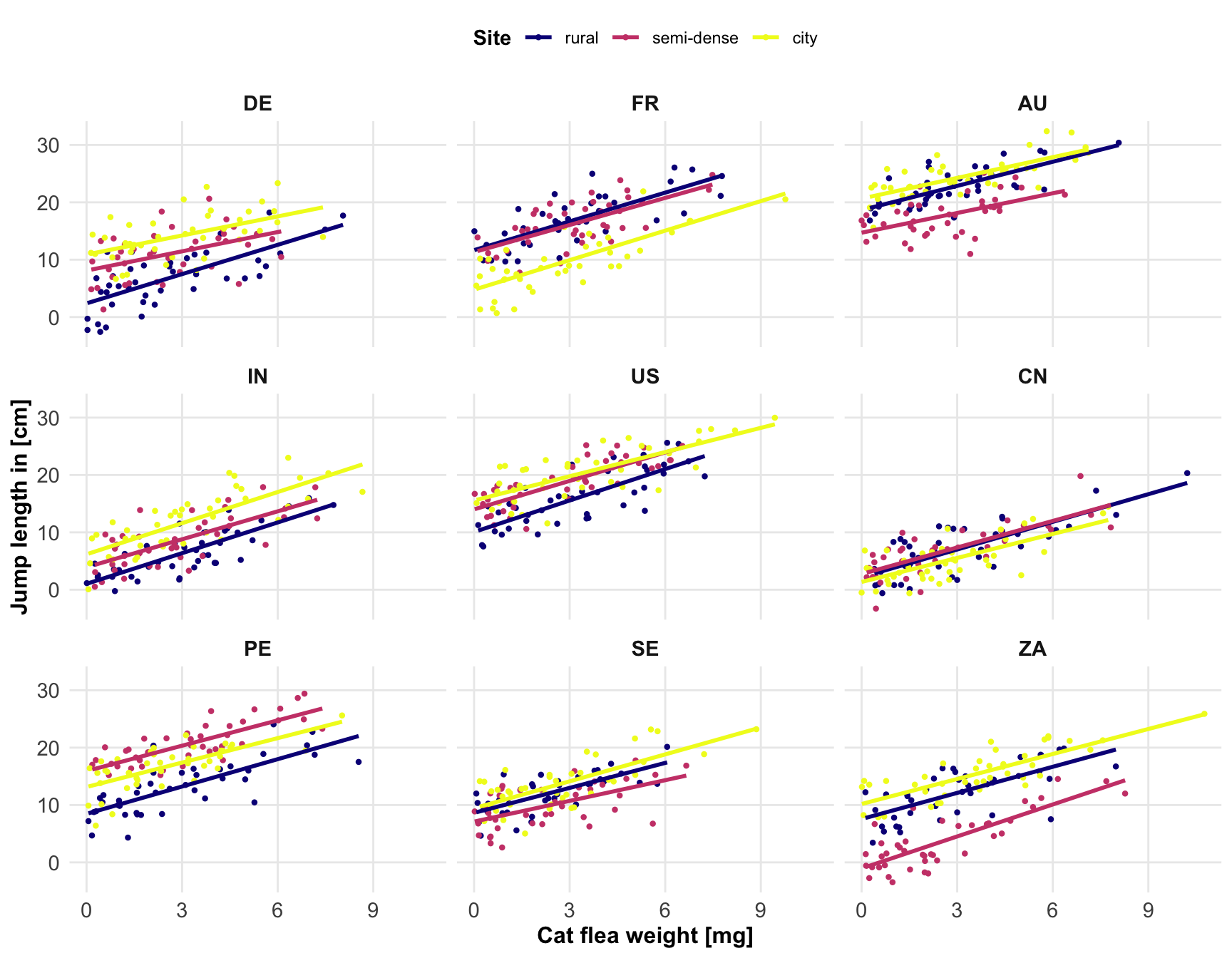
### International study
Degree of Urbanization of the United nations (rural as low-dense areas, town as semi-dense areas, cities as high-dense areas)
```{r}
#| echo: false
#| message: false
#| warning: false
#| label: fig-chap-13-worldmap
#| fig-align: center
#| fig-height: 2.5
#| fig-width: 7
#| fig-cap: "foo **(A)** foo **(B)** foo"
pacman::p_load(sf, rnaturalearth, rnaturalearthdata)
ne_countries(scale = "medium", returnclass = "sf") |>
mutate(my_selection = ifelse(iso_a2_eh %in% c("DE", "FR", "AU",
"IN", "US", "CN",
"PE", "SE", "ZA"),
1, 0)) |>
ggplot(aes(fill=as_factor(my_selection))) +
geom_sf() +
theme_void() +
scale_fill_viridis(option = "plasma", discrete = TRUE) +
theme(legend.position = "none") +
coord_sf(ylim = c(-50, NA))
```
ODer das ganze mal mit Bodylength?
```{r}
n_obs <- 41
jump_international_grid <- expand_grid(country = 1:9) |>
  mutate(mean_country = rnorm(9, 0, 4)) |>
  expand_grid(site = 1:3) |>
  mutate(mean_site = rnorm(27, 0, 4)) |>
  expand_grid(rep = 1:n_obs) |>
  mutate(bodyweight = abs(rnorm(n = (9*3*n_obs), 2.5, 2.5)),
         jumplength = 10 + 1.5 * bodyweight + mean_country + mean_site + rnorm(n = (9*3*n_obs), 0, 3))
```
DE = Germany
FR = France
IN = India
US = United States
CN = China
AU = Australia
PE = Peru
SE = Sweden
ZA = South Africa
```{r}
jump_international_tbl <- jump_international_grid |>
  select(bodyweight, country, site, jumplength) |>
  mutate(country = factor(country, labels = c("DE", "FR", "AU",
                                              "IN", "US", "CN",
                                              "PE", "SE", "ZA")),
         site = factor(site, labels = c("rural", "semi-dense", "city"))) |>
  mutate_if(is.numeric, round, 2)
```
```{r}
#| echo: false
#| message: false
#| warning: false
#| label: fig-chap-13-mixed
#| fig-align: center
#| fig-height: 7
#| fig-width: 9
#| fig-cap: "foo **(A)** foo **(B)** foo"
jump_international_tbl |>
ggplot(aes(bodyweight, jumplength, color = site)) +
theme_book() +
geom_point2() +
geom_smooth(method = "lm", se = FALSE) +
facet_wrap(~ country) +
scale_color_viridis(discrete = TRUE, option = "plasma") +
labs(x = "Cat flea weight [mg]", y = "Jump length in [cm]",
color = "Site")
```
```{r}
library(lme4)

lmer(jumplength ~ bodyweight + (site|country), data = jump_international_tbl)
c("#0D0887FF", "#5402A3FF", "#8B0AA5FF", "#B93289FF",
  "#DB5C68FF", "#F48849FF", "#FEBC2AFF", "#F0F921FF")
```
## Alternatives
Further tutorials and R packages on XXX
```{r}
expand_grid(obs = c(1, 3, 2)) |>
  rowwise() |>
  mutate(foo = list(expand_grid(1:obs))) |>
  unnest(cols = c(foo))
```
## Glossary
term
: what does it mean.
## The meaning of "Models of Reality" in this chapter.
- itemize with max. 5-6 words
## Summary
## References {.unnumbered}