12 It started with a line
Last modified on 08. January 2026 at 13:50:54
“It started with a
kissline; […] How could I resist?” — It Started With A Kiss by Hot Chocolate
In statistics, everything is about a line. This is also a lie. More precisely, in parametric statistics, everything is about a line. In a later chapter, we will also explore nonparametric statistical analysis, which is different but somewhat outdated. We have better tools on your shelves to solve problems that were previously solved using nonparametric approaches.
12.1 Geometry in statistics
Before we go any deeper into statistics, we need to either learn or review some geometry. We need to understand what a line is and how this concept differs in statistics. I will then explain the geometry of a square and the square root. You should be familiar with what both look like in a visualisation. We will revisit such geometries repeatedly. Ultimately, we will bring them together. A line can be expressed as a square. This is a key concept in statistics.
12.1.1 The square and the root
“What you see, well, you might not know; You get the feelin’, comin’ after the glow” — The joker & the thief by Wolfmother
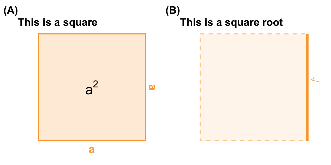
If you have never studied statistics before, or have only covered the basics, you may be surprised to learn that everything in statistics revolves around squares. However, this is only true for parametric statistics, which is where we want to start. In the following figure on the left side, you can see a square. A square has the same side length \(a\) on all sides, as well as a square area \(a^2\). If we want to find the side length of a square and only know its area, we can take the square root \(\sqrt{\phantom{a}}\) shown on the right side. This is a simple geometry, but an important one to remember. We will need to refer to squares repeatedly throughout this book.
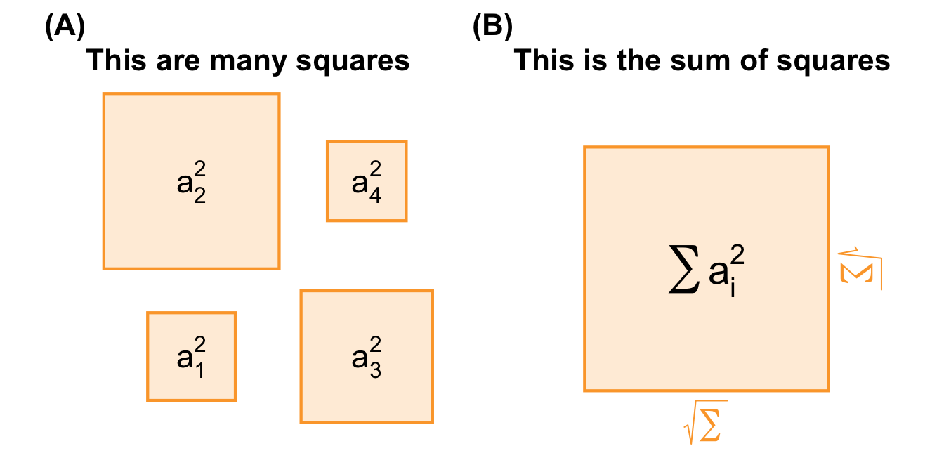
Now, let’s assume that there are lots of squares. Where these squares originate is not currently important. We have these squares and want to summarise them. A standard statistical procedure is to calculate the area of each square and then add up the areas. We call this new square the sum of squares. The sum of the squares is used so often that it is abbreviated to SS.
The following figure shows four squares labelled \(a_1, ..., a_4\) on the left. Each square has its own area, labelled \(a_1^2, ..., a_4^2\). In order to work with these squares, we will now add up their areas. The sum of the squares is shown on the right. The square root describes the length of the side of the sum of squares. We will use the sum of squares and the square root of the sum of squares repeatedly in our further analysis. They may not appear under the same names, but we will see the squares again.
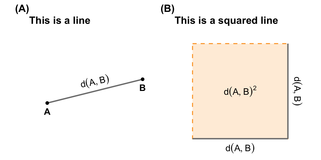
So far, this has not been very complicated. You might already remember the geometry from seeing a square. The tricky part is that we will work with mathematical expressions that are essentially squares, but don’t look like them. Now let’s combine a line with a square. Or answer the question of why a line can be expressed by a square.
12.1.2 The line as a square
12.1.3 The hunter and the rabbit
“Statistics is: When the hunter misses the rabbit once to the left and once to the right, on average the rabbit is dead.” — Mike Krüger, German comedian
I first came across the joke on Tweedback, a tool for anonymous feedback in lectures. One student had written the joke, which intrigued me. At first, I could not understand why. Then I understood the deeper meaning. In statistics, it’s all about lines. Or lines through points. A gunshot is a line. A mean is a line. Single shots deviate from the average shot, as do single observations from the mean. If we measure the distance from the mean to each observation, we will get positive and negative values. Ultimately, these values would sum to zero. I don’t believe for a moment that the comedian truly understands the depth of the joke from a statistical perspective.
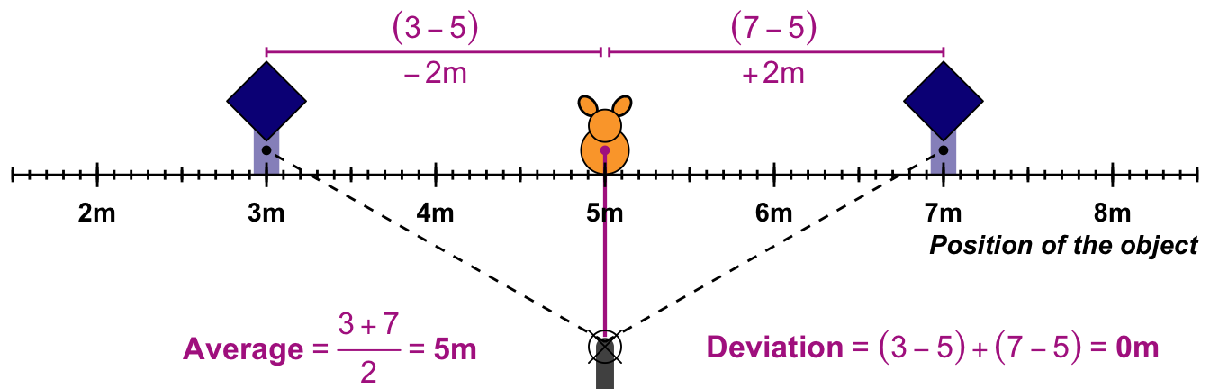
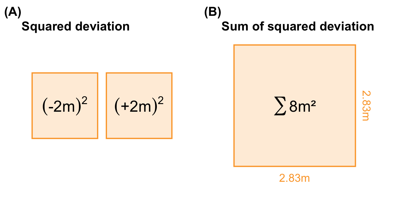
In the following Figure 12.4, I have illustrated the example with some numbers. The rabbit is sitting at position 5m. The hunter shoots at \(3m\), which is \(-2m\) to the left. The second shot goes to the right, at \(7m\), which is a deviation of \(+2m\). We can now calculate the average of the two shots. This is equal to \(5m\). The hunter hits. When we calculate the deviation, we get zero: \((-2) + (+2) = 0\). Therefore, the whole hunt of two shots has no deviation at all. This is wrong. Our model of reality tells us something completely different compared to what our hunter experienced. Therefore, we need a better model.
12.2 Normal distributed data
“Can’t explain all the feelings that you’re making me feel; I believe in a thing called
lovenormality.” — I Believe in a Thing Called Love by The Darkness
12.3 Glossary
- term
-
what does it mean.
12.4 The meaning of “Models of Reality” in this chapter.
- itemize with max. 5-6 words