```{r echo = FALSE, warning = FALSE, message = FALSE}
source("init.R")
source("images/part_0/part_0_model.R")
```
# Overview {#sec-what-is-a-model}
*Last modified on `r format(fs::file_info("chapter-53-overview.qmd")$modification_time, '%d. %B %Y at %H:%M:%S')`*
> *"A quote." --- Dan Meyer*
Imagine you are standing on a globe but still believe it is flat. You are standing on solid ground, with boiling rocks a few kilometers below you. A few kilometers above, you cannot breathe anymore. You are not moving, but the Earth is moving at speeds of up to 828,000 km/h, depending on the reference point. Your reality is a serious misinterpretation.
## What is a model in statistics?
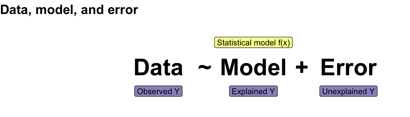
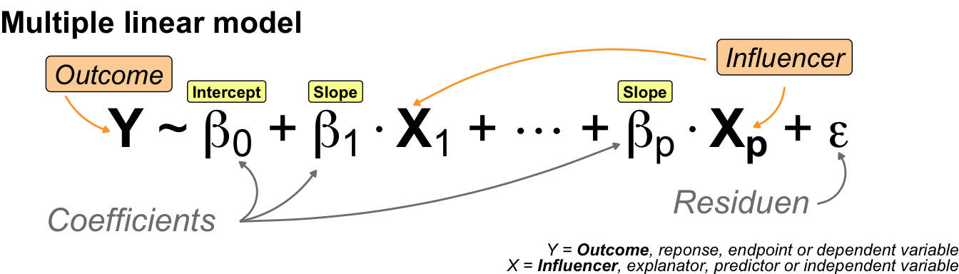
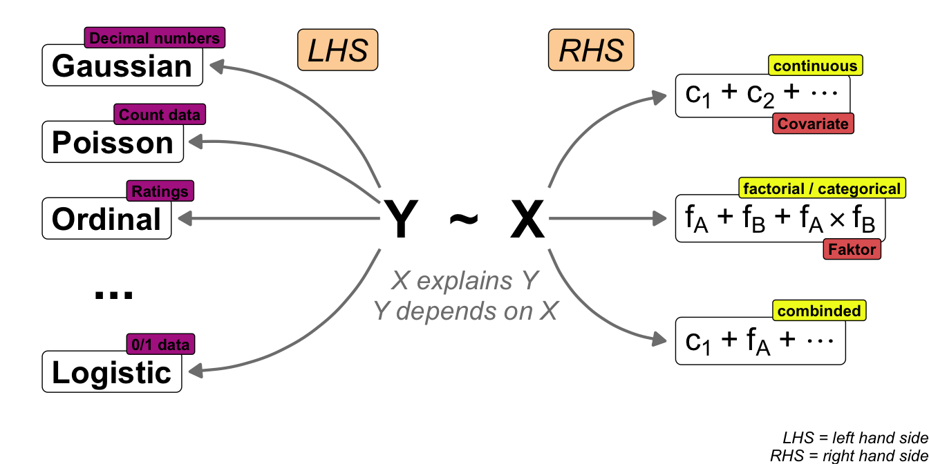
I would like to start with a simple example of a statistical model. Perhaps you would like to see a more concrete example of a model. But first, I will show you the most general form of a statistical model. The model is simple and contains only two terms combined with a tilde. The following @fig-model-general shows how the left-hand side and the right-hand side are connected.
```{r}
#| message: false
#| echo: false
#| warning: false
#| fig-align: center
#| fig-height: 1.75
#| fig-width: 7
#| fig-cap: "Visualisation of a theoretical statistical model with respect to the programming language R, with the outcome shown on the left-hand side (LHS) and the influencer pictured on the right-hand side (RHS). The two terms are combined by a tilde."
#| label: fig-model-general
p_lhs_rhs
```
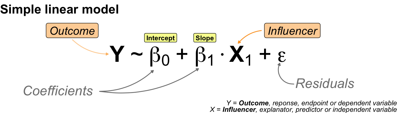
On the left-hand side (*LHS*) we find the outcome. The result of an experiment is called the **outcome**. The outcome is the measured value. Sometimes, using these words can cause you confusion, but for now we'll stick to the idea that the result of something is measured in an experiment. We will discover the outcome on the y-axis later on. Therefore, we abbreviate the outcome to Y. On the right side (*RHS*), you will find the **influencer**. The influencer is the thing we are trying to change in the experiment. If you change the influencer, the statistical model will show you the change in the outcome. As the change will be on the x-axis, we abbreviate the influencer to X. More often than not, we have one outcome and multiple influencers.
The world would be much easier, if there would be only one term for the measures y-values and the influencial values on the x-axis. But this is not true. Each scientific field has its own wording and the wording is changing, if you change the algorithm. So it is a real mess. I decided to use the words outcome and influencer for the y-values and x-values throughout the book for the general usage.
| Name | Symbol | Description |
|:----------------------|:------:|:----------------------------------------|
| **outcome**, response, endpoint, dependent variable | $y$ | *The right-hand side (abbr. RHS) of the model. Describing the values measured in an experiment or study. The majority of statistical models should typically have only one outcome variable.* |
| **influencer**, influential variable, risk factor, fixed effect, independent variable | $x$ | *The left-hand side (abbr. LHS) of the model. Describing the influential variables in an experiment or study. A statistical model can include more than one influencer.* |
: Table of terms used in the statistical modelling for the left hand side and right hand side. The terms in bold are used here. Depending on the scientific background, the usage of these terms can vary widely. {#tbl-names-regression}
text
| Name | Symbol | Description |
|:----------------------|:------:|:----------------------------------------|
| **explanator**, explanatory variable | $x$ | **Explanation** --- *The influencer is used to describe or explain the change of the outcome.* |
| **predictor**, predictive variable | $x$ | **Prediction** --- *The influencer is used to predict values of the outcome.* |
| **focal explanator**, **focal predictor**, focal variable | $x$ | **Main effect** --- *In a model with multiple influencers, the focal variable is the variable of primary interest.* |
: Table of terms used in the statistical modelling. The terms in bold are used here. Depending on the scientific background, the usage of these terms can vary widely. {#tbl-names-regression-2}
text
| Name | Symbol | Description |
|:----------------------|:------:|:----------------------------------------|
| **covariate**, covariable | $c$ | **Continuous** $\boldsymbol{x}$ --- *The influencer is a numeric variable with continuous values.* |
| **factor A**, factorial variable, categorical variable | $f_A$ | **Categorical** $\boldsymbol{x}$ --- *The influencer is discrete, functioning as a grouping variable, such as an experimental group or a treatment.* |
| **levels**, groups, treatment groups | $A.1$ to $A.j$ | *The discrete groups included in one factor* $\boldsymbol{f_A}$. |
: Table of terms used in the statistical modelling. The terms in bold are used here. Depending on the scientific background, the usage of these terms can vary widely. {#tbl-names-regression-3}
A sentence why we use $y$ and not $x$ for mean and other stuff.
@mccullagh2002statistical [What is a statistical model?](https://projecteuclid.org/journals/annals-of-statistics/volume-30/issue-5/What-is-a-statistical-model/10.1214/aos/1035844977.pdf)
@appleton1995we [What do we mean by a statistical model?](https://onlinelibrary.wiley.com/doi/abs/10.1002/sim.4780140209?casa_token=jLDogF46zS8AAAAA%3AKOKHMTgbj4gK8ayVXmT1GaXq7slv9i3VGqzA184yydwKUjsDIszepgOaeMQc_L5hRY-TpLZvgDDIdDea)
@hand2019purpose [What Is the Purpose of Statistical Modeling?](https://hdsr.mitpress.mit.edu/pub/9qsbf3hz/release/2?from=603&to=744)
@spanos2006statistical [Where do statistical models come from? Revisiting the problem of specification](https://arxiv.org/pdf/math.ST/0610849)
@gilchrist1984statistical [Statistical modelling](https://nzdr.ru/data/media/biblio/kolxoz/M/MV/MVsa/Gilchrist%20W.%20Statistical%20modelling%20with%20quantile%20functions%20(Chapman,%202000)(ISBN%201584881747)(317s)_MVsa_.pdf)
```{r}
#| echo: false
#| message: false
#| warning: false
#| label: fig-scatter-modeling-R-01
#| fig-align: center
#| fig-height: 5
#| fig-width: 15
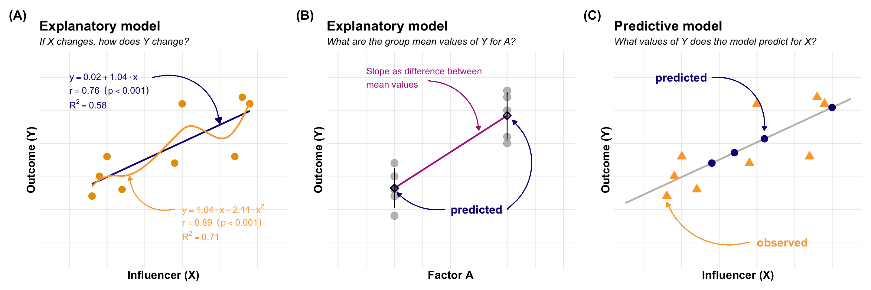
#| fig-cap: "Visualisation of the causal and predictive model in statistical modelling for a simple model. In all cases, the outcome $Y$ is normally distributed. **(A)** *Explanatory model:* How does the outcome y change when the continuous influencer $X$ changes? What is the numerical relationship between $Y$ and $X$? This is a question about the slope of the line. **(B)** *Explanatory model:* How does the outcome $Y$ change when the categorical influencer as factor $f_A$ changes? What is the numerical relationship between $Y$ and $f_A$? This is a question about the slope of the line and the difference between the predicted means of each group. **(C)** *Predictive model:* If $Y$ and $X$ have been measured, what are the values of $Y$ for new $X$ values? Can we use the influencer $X$ to predict new $Y$ outcomes?"
simple_tbl <- tibble(jump_length = c(1.2, 1.5, 1.8, 1.3, 1.7, 2.6, 1.8, 2.7, 2.6),
weight = c(0.8, 0.9, 1, 1.2, 1.9, 2, 2.7, 2.8, 2.9),
grp = as_factor(c("Gruppe 1", "Gruppe 1", "Gruppe 1", "Gruppe 1", "Gruppe 2", "Gruppe 2", "Gruppe 2", "Gruppe 2", "Gruppe 2")))
fit_1 <- lm(jump_length ~ weight, data = simple_tbl)
pred_tbl <- bind_rows(mutate(simple_tbl, status = "observed"),
tibble(weight = c(1.7, 1.4, 2.1, 3.0),
jump_length = predict(fit_1,
newdata = tibble(weight)),
status = "predicted")) |>
mutate(status = factor(status, levels = c("predicted", "observed")))
group_tbl <- tibble(f = gl(2, 5, labels = c("A.1", "A.2")),
y = c(0.9, 1.5, 1.7, 1.3, 1.2,
2.7, 2.5, 2.8, 2.1, 2.0))
group_fit <- lm(y ~f, data = group_tbl)
p_explanatory_fct_model <-
group_tbl |>
ggplot(aes(as.numeric(f), y)) +
theme_minimal() +
geom_line(aes(y = predict(group_fit)), color = "#B12A90FF", linewidth = 1) +
geom_point(color = "gray50", alpha = 0.5, size = 4) +
stat_summary(fun.data=mean_sdl, , fun.args = list(mult = 1),
geom="pointrange", shape = 23,
fill = c("#0D088780", "#0D088780"), size = 0.75) +
annotate("text", x = 0.75, y = 3, hjust = "left", color = "#B12A90FF", size = 4,
label = "Slope as difference between\nmean values") +
geom_curve(x = 1.3, y = 2.95, xend = 1.75, yend = 2.2,
arrow = arrow(length = unit(0.02, "npc"), type = "closed"),
curvature = -0.4, color = "#B12A90FF") +
annotate("text", x = 1.5, y = 1, hjust = "left", color = "#0D0887FF",
size = 5, label = "predicted", fontface = 2) +
geom_curve(x = 1.45, y = 1, xend = 1.025, yend = 1.25,
arrow = arrow(length = unit(0.02, "npc"), type = "closed"),
curvature = -0.25, color = "#0D0887FF") +
geom_curve(x = 2, y = 1, xend = 2.05, yend = 2.35,
arrow = arrow(length = unit(0.02, "npc"), type = "closed"),
curvature = 0.5, color = "#0D0887FF") +
ylim(0.25, 3.25) +
xlim(0.5, 2.5) +
theme(legend.position = "none",
axis.text.x = element_blank(),
axis.text.y = element_blank(),
axis.text = element_text(size = 12),
plot.subtitle = element_text(size = 12, face = "italic"),
title = element_text(size = 14, face = "bold")) +
labs(x = "Factor A", y = "Outcome (Y)",
title = "Explanatory model",
subtitle = "What are the group mean values of Y for A?")
p_explanatory_cov_model <-
ggplot(filter(pred_tbl, status == "observed"),
aes(weight, jump_length, color = status, shape = status)) +
labs(x = expression(x[1]), y = "y", color = "", shape = "",
title = "Explanatory model",
subtitle = "If X changes, how does Y change?") +
geom_point(size = 4) +
theme_minimal() +
scale_color_okabeito() +
xlim(0.25, 3.25) + ylim(0.25, 3.25) +
theme(legend.position = "none",
axis.text.x = element_blank(),
axis.text.y = element_blank(),
plot.subtitle = element_text(size = 12, face = "italic"),
axis.text = element_text(size = 12),
title = element_text(size = 14, face = "bold")) +
annotate("text", x = 0.5, y = 3, hjust = "left", color = "#0D0887FF", size = 4,
label = TeX(r"($y = 0.02 + 1.04 \cdot x$)")) +
annotate("text", x = 0.5, y = 2.8, hjust = "left", color = "#0D0887FF", size = 4,
label = TeX(r"($r = 0.76\; (p<0.001)$)")) +
annotate("text", x = 0.5, y = 2.6, hjust = "left", color = "#0D0887FF", size = 4,
label = TeX(r"($R^2 = 0.58$)")) +
geom_curve(x = 1.6, y = 3, xend = 2.5, yend = 2.3,
arrow = arrow(length = unit(0.03, "npc"), type = "closed"),
curvature = -0.5, color = "#0D0887FF") +
geom_smooth(method = "lm", se = FALSE, color = "#0D0887FF") +
geom_smooth(method = "loess", se = FALSE, color = "#FCA636FF") +
annotate("text", x = 2, y = 1, hjust = "left", color = "#FCA636FF", size = 4,
label = TeX(r"($y = 1.04 \cdot x - 2.11 \cdot x^2$)")) +
annotate("text", x = 2, y = 0.8, hjust = "left", color = "#FCA636FF", size = 4,
label = TeX(r"($r = 0.89\; (p<0.001)$)")) +
annotate("text", x = 2, y = 0.6, hjust = "left", color ="#FCA636FF", size = 4,
label = TeX(r"($R^2 = 0.71$)")) +
geom_curve(aes(x = 1.9, y = 1, xend = 1.3, yend = 1.5),
arrow = arrow(length = unit(0.02, "npc"), type = "closed"),
curvature = -0.5, color = "#FCA636FF") +
labs(x = "Influencer (X)", y = "Outcome (Y)")
p_predcited_cov_model <- ggplot(pred_tbl, aes(weight, jump_length, color = status, shape = status)) +
stat_smooth(method = "lm", se = FALSE, fullrange = TRUE,
color = "gray", linetype = 1) +
labs(x = expression(x[1]), y = "y", color = "", shape = "",
title = "Predictive model",
subtitle = "What values of Y does the model predict for X?") +
geom_point(size = 4) +
theme_minimal() +
scale_color_viridis(discrete = TRUE, option = "plasma", end = 0.8) +
xlim(0.25, 3.25) + ylim(0.25, 3.25) +
theme(legend.position = "none",
axis.text.x = element_blank(),
axis.text.y = element_blank(),
axis.text = element_text(size = 12),
plot.subtitle = element_text(size = 12, face = "italic"),
title = element_text(size = 14, face = "bold")) +
annotate("text", x = 0.65, y = 3, hjust = "left", color = "#0D0887FF",
size = 5, label = "predicted", fontface = 2) +
annotate("text", x = 2, y = 0.5, hjust = "left", color = "#FCA636FF",
size = 5, label = "observed", fontface = 2) +
geom_curve(x = 1.4, y = 3, xend = 2.1, yend = 2.2,
arrow = arrow(length = unit(0.02, "npc"), type = "closed"),
curvature = -0.5, color = "#0D0887FF") +
geom_curve(x = 1.9, y = 0.5, xend = 0.8, yend = 1.1,
arrow = arrow(length = unit(0.02, "npc"), type = "closed"),
curvature = -0.4, color = "#FCA636FF") +
labs(x = "Influencer (X)", y = "Outcome (Y)")
p_explanatory_cov_model + p_explanatory_fct_model + p_predcited_cov_model +
plot_layout(ncol = 3) +
plot_annotation(tag_levels = 'A', tag_prefix = '(', tag_suffix = ')') &
theme(plot.tag = element_text(size = 16, face = "bold"))
```
## Theoretical background
```{r}
#| message: false
#| echo: false
#| warning: false
#| fig-align: center
#| fig-height: 2
#| fig-width: 7
#| fig-cap: "foo"
#| label: fig-model-in-R-2
p_model_abstract
```
```{r}
#| message: false
#| echo: false
#| warning: false
#| fig-align: center
#| fig-height: 2
#| fig-width: 7
#| fig-cap: "foo"
#| label: fig-model-in-R-4
p_model_exp_simple_reg
```
```{r}
#| message: false
#| echo: false
#| warning: false
#| fig-align: center
#| fig-height: 2
#| fig-width: 7
#| fig-cap: "foo"
#| label: fig-model-in-R-5
p_simple_model
```
```{r}
#| message: false
#| echo: false
#| warning: false
#| fig-align: center
#| fig-height: 2
#| fig-width: 7
#| fig-cap: "foo"
#| label: fig-model-in-R-6
p_mult_model
```
```{r}
#| message: false
#| echo: false
#| warning: false
#| fig-align: center
#| fig-height: 2
#| fig-width: 7
#| fig-cap: "foo"
#| label: fig-model-in-R-7
p_lhs_rhs_simple_r
```
```{r}
#| message: false
#| echo: false
#| warning: false
#| fig-align: center
#| fig-height: 2
#| fig-width: 7
#| fig-cap: "foo"
#| label: fig-model-in-R-8
p_lhs_rhs_mult_r
```
```{r}
#| message: false
#| echo: false
#| warning: false
#| fig-align: center
#| fig-height: 2.5
#| fig-width: 9.5
#| fig-cap: "foo"
#| label: fig-model-in-R-9
p_regression_wording
```
```{r}
#| message: false
#| echo: false
#| warning: false
#| fig-align: center
#| fig-height: 3.5
#| fig-width: 7
#| fig-cap: "foo"
#| label: fig-model-in-R-10
p_lhs_rhs_detail
```
```{r}
#| message: false
#| echo: false
#| warning: false
#| fig-align: center
#| fig-height: 2.75
#| fig-width: 7
#| fig-cap: "foo"
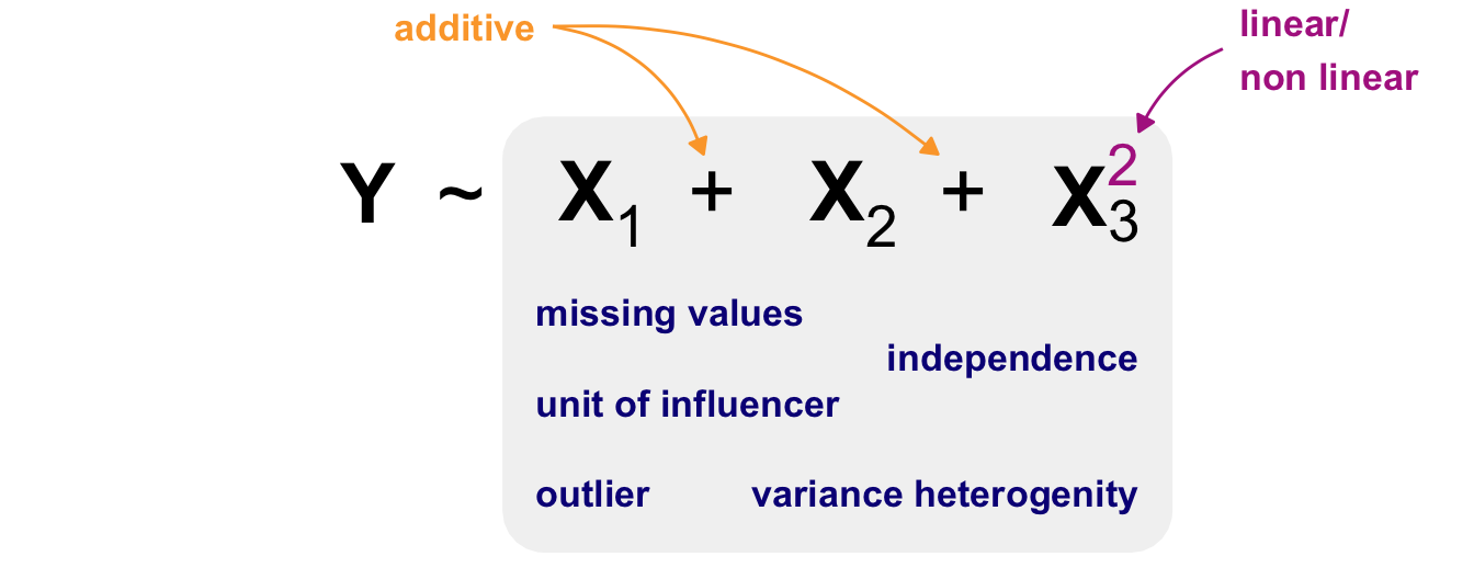
#| label: fig-model-in-R-11
p_problem_x
```
> *"Twistin', shake it, shake it, shake it, shake it, baby; Hey, we gonna Loop de Loop Shake it out, baby; Hey, we gonna Loop de La" --- [The Blues Brothers (1980) -- Shake a Tail Feather](https://www.youtube.com/watch?v=qdbrIrFxas0)*
## R packages used
## Data
## Alternatives
Further tutorials and R packages on XXX
## Glossary
term
: what does it mean.
## The meaning of "Models of Reality" in this chapter.
- itemize with max. 5-6 words
## Summary
## References {.unnumbered}