
2 What is data?
Last modified on 03. May 2026 at 18:54:20
“The limits of my language mean the limits of my world.” — Ludwig Wittgenstein
Emma sat on the wooden stage. She need time to recover from what she had seen behind the curtains. What she had seen beneath the wood had now become reality. Dust danced in the light. Single light beams hit some dust particles from time to time and exploded into golden rain. Sparkles dropped on the wood.
“How is gold made?” Emma asked.
“This was a long break. I’m a bit surprised by your question. I thought we should discuss your findings from behind the stage. Not gold.” Jeff answers from his seat on the left.
“Gold cannot be formed through fusion in a star. This is only possible up to iron. You need a supernova or a collision of two neutron stars.” Emma spoke absently into the darkness.
“Interesting topic. Was this observed? The collision of two neutron stars and the resulting gold spewing out,” Jeff laughed.
“No, it was a computer simulation. Artificial data, if you will.” Emma looked around. She decided that it was time to begin the play.
“Then it’s not real, and it’s not an explanation for me at all.” Jeff stated.
“But the simulation was based on real observations.” Emma stood up and started building the scene for the play.
2.1 What is observed?

Can we observe anything? What does it mean to observe? We see things, but our vision is already influenced by our understanding of what they are. Additionally, by naming things and processes, we are already following a theory. “The sun is rising” is a popular example of a saying connected with the geocentric theory, which states that the Earth is at the center of the solar system. Therefore, our language is already influenced by our observations. We cannot speak about something we observe without giving the observation some meaning. It is possible, but it demands a high level of concentration.
This book requires a highly specific type of observation. We need data. Very rarely is any observation we make based on first-hand data. For example, if you look outside your window and observe a bird, you will learn some information about it. But is this data? No, it is just information. Data is information, but structured information. Data is a type of observation that is stored in a specific way. We translate observations and information about them into a set of numbers. Not every observation can be represented as a number in a data sheet or table. As their names suggest, data sheets and tables are two-dimensional. A sheet is a type of paper on which organised observations can be written down. The same is true for a table. It is a structured type of observation.
2.2 What is data?
We will now think about data. This will happen after we have discussed the science in the chapter. It will also happen if you have skipped the chapter entirely. What is data? If you had asked me when I was a teenager, I would have referred to Star Trek: The Next Generation and Commander Data. He was an android without any emotions. Pure objectivity. He was an artificial being. However, this is not the type of data we want to discuss. We want to discuss data that has been observed and measured. Furthermore, our data is numeric or has a numeric counterpart. We use descriptive words, but rarely. Later on, we want to run algorithms and calculations with our data. Therefore, the data must be open to calculations.
Data are observations represented by numbers and letters. Can we use data in any format? No, you cannot. There is a general format for how data should be stored. In our case, we have observations in the rows and variables of measurement in the columns. There can only be one observation per row. This format is called the long format. Another possibility is the wide format, where the observations are scattered around and do not share the same rows. The wide format may be useful for time series, but I do not recommend it.
The following Figure 2.3 shows a typical data set used in data science and statistics. It is also typical for those working in the life sciences. The matrix has \(n\) rows and \(p\) columns. To select a cell, we can write the row and column information in brackets. The rows are indicated by \(i\) and the columns by \(j\). This is a simple way of extracting information from a data table. However, these manipulations are not normally used anymore because they are very error-prone. This is a simple yet powerful way of storing information. We translate our observations into numbers and letters, which we then put into a two-dimensional matrix.
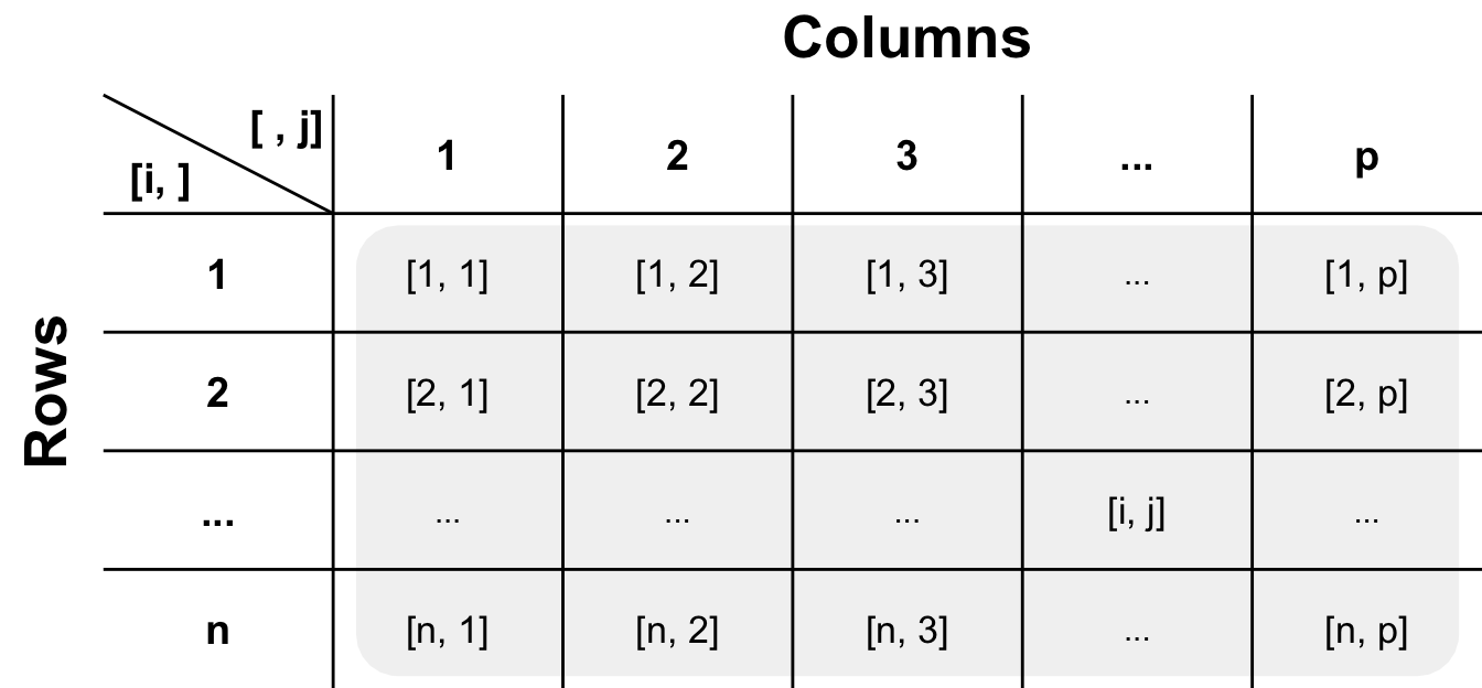
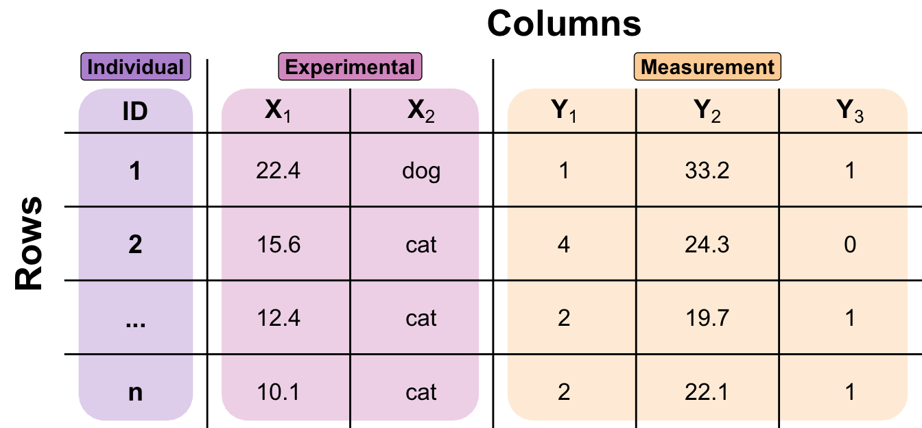
Figure 2.4 might be interesting, but it is not very helpful in the daily working process. Therefore, I will show you an annotated data table with example observations labelled with numbers and letters. The first columns contain an identifier for each observation, or ID. I always include one in my data sets because I always want to know which individual is which. This is even more important when working with time series or repeated measurements. After the ID column, we find the experimental variables. We can also refer to these as ‘X’ variables, as we will plot them on the x-axis in our visualizations later on. We will often set the experimental variables before we start the experiment. Then, we find the measurements on the individuals. These variables are called outcomes or ‘Y’ variables, as they will be the variables on our y-axis later on. The terminology used varies from scientific field to scientific field. I will therefore talk about terminology in a separate chapter later on.
Can we live with this two-dimensional representation of data? Not really. If you look at different fields, you will find a variety of other data tables. In genetics, we do not have data sets of this kind when we look at thousands of genes. Therefore, we have at least two data files: One contains all the information on the patients or individuals, and the other contains all the genetic information. Most of the time, the genetic file is saved in a transposed form. This means that the variables or genes are in the rows and the individuals are in the columns. This is because it is easier to change rows in a data set than columns. This gives us an advantage when it comes to saving and manipulating the data. However, this makes it slightly more complicated to work with such data. Further, geology has its own data format, while other fields use different ways of storing data. Storage methods sometimes depend on the analysis software used or the storage and calculation capacities required.
Here, we will focus on the presented data set in Figure 2.4, making some modifications to the columns if we are working with time series or repeated measurements. However, we will stick to one data set and will not consider complicated representations. We will talk about the experimental variables and the different types of measurements, both of which are represented by different numbers and letters. There are still many topics to consider if we want to work with data to obtain information and knowledge. In the following sections, we will cover different attributes and limitations of data that are important for successful work.
2.3 Meta information of data
The data seems easy enough. We have a two-dimensional table with numbers and letters. That could be it. However, there are some things to consider. Information is often hidden in data. Where does the data come from? What are the internal generation processes? Are there unknown or known structures beneath the numbers and letters that cannot be seen by the row and column names?
First, we need to consider the source of the data. Depending on where you obtain your data, there may be more regularities to consider than in other fields.
Second, we must discuss how the data is generated. Are you conducting a controlled experiment where you only change one influential variable and observe what happens? Or are you doing nothing and only observing the data? Does your role in the generation process play an important role?
Third, we would like to discuss the replication. We need replications in our data in order to perform statistical analyses later on. However, there are two types of replication. They can appear similar in a dataset, but they have a significant impact on your analysis and the answers to your questions.
Is the data valid? This may seem like a simple question, but it is sometimes very important. If you are a statistician working with data, your possibilities are limited. Often, you are not an expert in the field in which you are conducting the analysis. You could argue that men should, on average, be larger than women. However, if the data is more specific, you need help to determine its validity.
Next, we will examine artificial or simulated data. This special type of data is used mainly in statistical research and teaching, and we will use it in this book. Non-statisticians should not use artificial data in their daily research to cheat their data sheets.
Is all this information lost or hidden? In a sense, yes, because if you don’t have any information on the generation process, or if you can only see some cryptic column names, it might be impossible for you to gain any deeper knowledge of the data. However, it is always possible to find a pattern in anything.
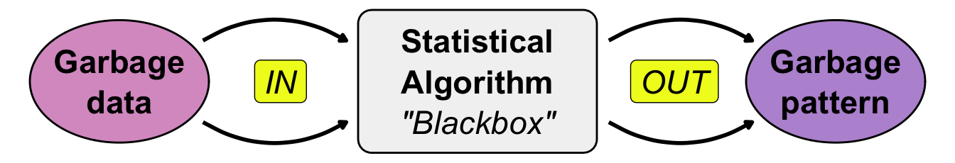
Garbage in garbage out
2.3.1 Source of data
Where does your data come from? Does it matter? Yes, because it has a huge influence on your work and how you share it. First, let’s define the different sources of data. One type is human data, such as blood samples or questionnaires. Humans can share information about social, economic, and other factors. Human data is often used in medicine and the social sciences. Then, we can examine data from animals. Mice are a special case because much basic research is conducted on mice before moving on to humans. The rest of the animal studies include all animals relevant to agriculture and leisure activities, such as dogs and horses. Naturally, there is a great deal of interest in chickens, pigs, and cows because of their role in food production. Finally, we have plants, including fungi and other plant-based sources. Our focus is mostly on crops that are interesting to agriculture, but the field is broad. On the sidelines, we have cell cultures, which have their own problems and limitations.
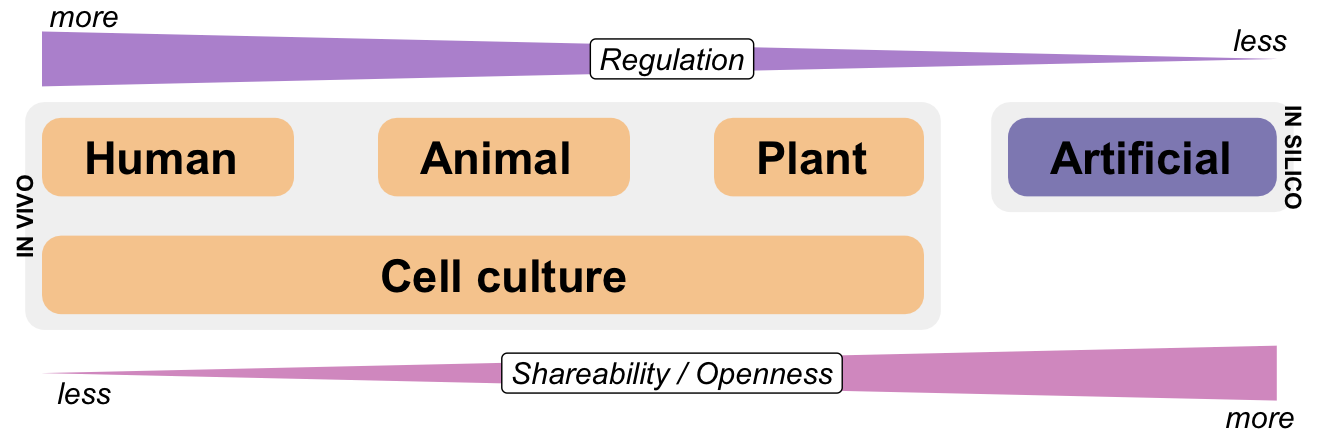
Figure 2.5 shows a visualization of the different sources of data and their connection to regulation and openness. We often refer to data from humans, animals and plants as in vivo data because it originates from living beings. This includes mice, which are the general animal model for humans. If artificial or simulated data is used in statistics, these data sources are referred to as in silico data. In my view and in the context of this book, artificial data is common, but this is a biased perspective on data. Most of the time, data is generated by experiments or observations rather than by algorithms. Nevertheless, human data is largely regulated. Human data cannot be shared openly. The same is partly true for animal models. Plant data and some types of cell cultures are easier to share. If you simulate your data, you can share it as freely as you like.
Finally, we must consider the ethical and cultural issues involved. You cannot do whatever you want with patients and animals. Depending on your location and nationality, the process of working with or sharing human or animal data is highly regulated. You may need an ethical vote from an Ethics Committee at your institution or approval for an animal experiment from a different committee. Sometimes cultural borders hinder work with specific animal breeds. All of this is beyond the scope of this book. If you are unsure whether your experiment can be conducted and data collected, please contact a statistician at your institution or a nearby university. As a general rule, never upload any human patient data, with or without personal identifiers, to an open database without consulting the relevant legal authorities first.
2.3.2 Experimental vs. observed data
There is a lot that could be written about experimental and observed data. The terminology can be a little confusing because ‘experimental data’ consists of observations that have been clearly recorded. Therefore, I prefer to refer to it as data that comes from a controlled experiment. Conversely, observed data is data generated without any influence from an experimenter. In this book, we will focus primarily on experimental data. However, many of the algorithms introduced can also be used with observed data. There are no real limitations to their application. The problem lies in interpretation. With experimental data, you know which influencers are changing because you are the one changing them. With observed data, however, you can never be sure whether you are observing correlation or causality because you are not controlling any of the influencing factors. If you are missing information, you may draw the wrong conclusions.
In a clinical context, we often refer to observed data as real-world data, which can come from anywhere. This can be data collected from wearable devices such as clocks and smartphones. It can also be collected from operations or other examinations of patients during normal clinical processes. This data is merely observed; there is no controlled assignment of patients to treatments or other controlled activities. In this context, we can also speak of experimental data from randomised clinical trials (RCTs) and observational data as real-world data from clinical routine.
We live in a data-driven world. Or, we could say that we live in an information-driven world. There is so much information available that we believe everything is clear and well known. Sometimes, however, we realise that this is not the case. We only have partial information in very specific areas where we gather it. Someone might think that weather forecasting should be easy. We have satellites, we know past temperatures, wind speeds and air pressure. Yet we still have problems predicting the weather a week in advance or thunderstorms a few hours in advance. We know that the conditions are right for a thunderstorm, but we only find out where it will build up once we observe it.
2.3.3 Biological vs. technical replication
When I first started studying statistics, I found the replications a little irritating. I was familiar with numbers and calculations from school mathematics lessons. There we had a formula or equation and I put in numbers to calculate something. I never did this more than once. Why should I calculate the same thing again and again? Why is there replication in statistical data? We need replication, because we need a probabilistic process to do statistics in science. By the probabilistic process we can then calculate probabilities. Without a probabilistic process and replication we cannot have any probabilities. Perhaps the explanation comes a little early, but we will revisit this topic throughout the book. It is important to remember here that we want to calculate probabilities. Therefore, we need replications in order to calculate these probabilities.
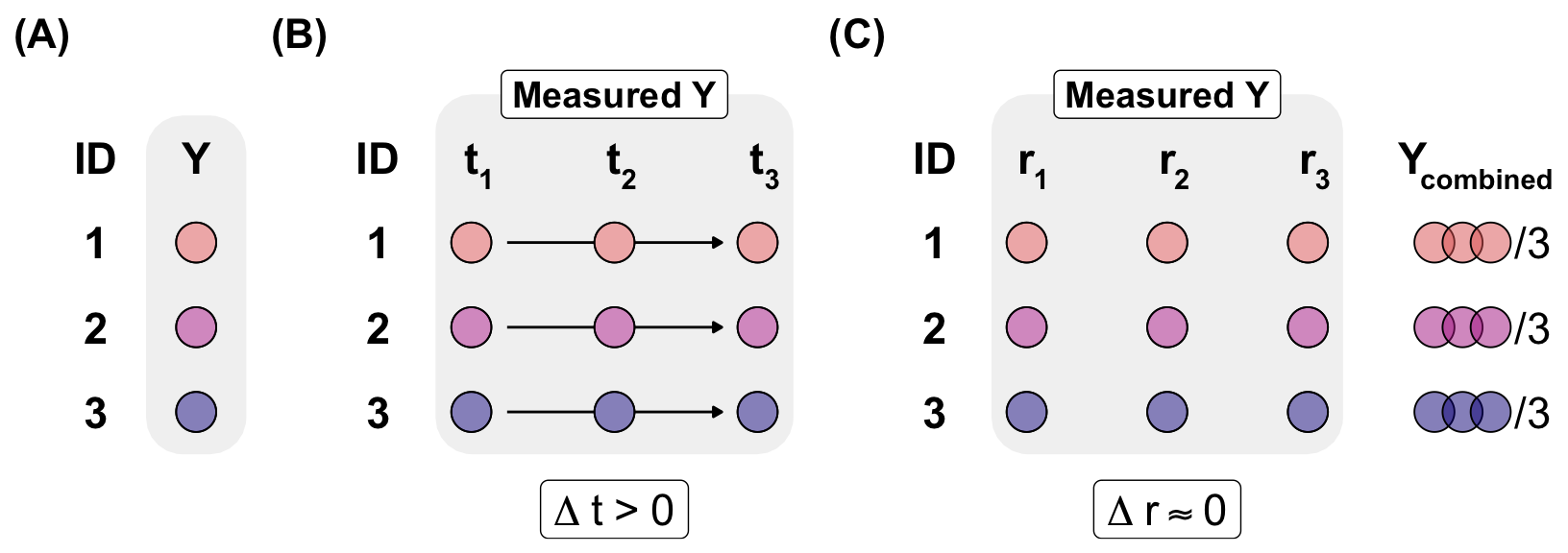
The following Figure 2.6 illustrates the various types of replication. In general, we divide replication into biological and technical replication. We are also able to conduct biological replication at many points in time. This may sound confusing, but the difference lies in the time between the measurements. Let us start with biological replication. We measure an outcome Y on different biological individuals. Depending on our research question, we might measure only a few individuals or hundreds to thousands. These individuals can be humans, plants or mice. Technical replication involves taking measurements many times on the same individual at the same time. This allows us to ensure that the measurement was correct. For example, you could take your body weight three times and then combine the three measurements to give one overall result. If a large amount of time passes between the individual measurements, we speak of a repeated measurement. In this case, we are still measuring the same individual, but at different points in time. We want to know how body weight changes in humans over weeks. This is a biological replication at different points in time.
Sometimes cell cultures can become a bit strange. Where is the statistical replication in the technical replication? If we replicate the same cell three times, we have a clone. This is not a biological replicate, which is usually considered a statistical replicate. We need variance to run our statistical algorithms. One solution would be to add or subtract a small random value, such as \(\pm0.001\), to each measured value, but I cannot recommend this approach. This solution is only feasible if nothing else is possible and a running statistical test is really necessary. In reality, our experimental design does not align with the statistical theory framework. You will need to design your experiment differently and repeat it.
NoteA word of caution: Should be all the values the same?
If you are new to science and experiments, you might think that the best outcome of a measurement would be the same value each time you measure something. In this case, you are muddling up biological and technical replication. If you measure the same thing on the same object, you should always get the same value. If you step on your personal scale three times in the morning, you should get the same value each time. However, if you, your potential partner and your offspring each step on the scale once, you should get three different body weight values.
Later in the book, we will run statistical algorithms that depend on a concept called ‘variance’. If you always measure the same value in your experiment, the variance will be zero. In this case, you will quickly realise that you need to divide your summary statistics of your data by the variance. However, if all the values are the same, you will divide by zero, which is a severe mathematical problem that will cause most algorithms to crash and return an error message.
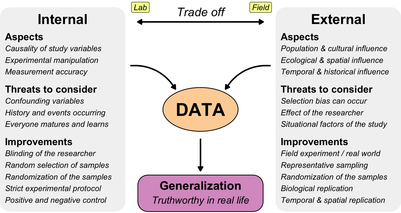
2.3.4 Internal and external validity
Can we trust the data we are working with? Is it valid, and what can we do with it? The answers to these questions depend on the information buried in the data. If we can find useful information in our data, we can use it to make decisions or predictions. However, these will only be useful for future events if past data can be connected to the future. Therefore, we want to examine the validity of our data. This is essentially meta-information about your data. There is no method of determining the validity of data alone. You cannot look at a data table and simply declare that the data is valid. You need additional information alongside the raw data tables.
For example, it is well known that men are generally larger than women. Therefore, we would expect male patients to be larger on average than female patients in a data set of patients. However, this is only partly true. The height distribution also depends on age, so in a clinical study of younger patients, the girls may be taller than the boys. Therefore, I would advise against using general rules without considering the context of the data.
Internal validity is often considered a prerequisite for external validity, as a experiment must first be true for its included observations before it can be generalized to the broader population.
NoteExamples of failures in internal validity
Why doesn’t my experiment work? Or why can’t other scientists reproduce my results? Why do I make observations that cannot be explained and still don’t feel real? There can be different reasons for this, and here I will give you three examples from my consulting work and literature to inspire you and give you food for thought.
- Moving plants
-
You might say that the biggest difference between plant, animal and human experiments is that plants cannot move, whereas animals can and humans run away. Therefore, you might assume that plants always stay in one place. This may be true for field experiments, but anything else that can move will move. Some strange things have happened in my many years of statistical consulting. For example, plants in pots move because the janitor had to do some repairs and thought he had put the plants back in the same spot. Plants move because visitors might rearrange them. This happened with pupils from a visiting class. They find it appealing to sort the pots in increasing order of plant height. Sometimes, even the tubes move the plants because they were in the wrong position, causing the plants to move when the tubes were moved.
- Mice with big ears
-
During another consultation, we observed strange patterns in the mice under observation. Large mice in particular exhibited unusual behaviour during the treatment regime. We started to investigate and found that one of the laboratory staff had been a little too practical. When there were more than nine mice to be numbered on the ears with a pen, she found it easier to write large two-digit numbers on the mice with larger ears. Intuitively, the mice with larger ears were also larger. Unknowingly, she had introduced a selection bias into the data. This was not due to laziness, as the writing was very neat and the selection process took much longer than randomly selecting a mouse and writing a number on its ear. This is a good example of the need for statistical education and experimental design, even among laboratory staff who mainly conduct experiments. If procedures become a cargo cult with no meaning, everyone will try to optimise the workflow at some point.
Electrified children
A final example comes directly from human science. Every new discovery opens up new possibilities for humanity. This is also true of the discovery of electricity. In 1912, the Swedish chemist Svante Arrhenius exposed newborn infants in an orphanage to high-frequency electric currents to see if they would become stronger1. This teaches us two things: first, that if not regulated, humans will do strange things to other humans. Ethics are fundamental to clinical studies. Secondly, parents do not want their children to be involved in such experiments. Therefore, Arrhenius had to use an orphanage as a source of participants. He thought that if there were no parents around, no one would intervene. Arrhenius was able to stimulate the growth and development of children using electricity. At first glance, this seems like a stunning result. However, there were always heroes around, and in this case, the nurses had placed the healthier babies in the electrified group and the weaker, malnourished ones in the control group.
https://pmc.ncbi.nlm.nih.gov/articles/PMC6188693/
https://en.wikipedia.org/wiki/External_validity
https://www.researchgate.net/profile/Jolaine-Draugalis/publication/260267611_Establishing_the_internal_and_external_validity_of_experimental_studies/links/56c2042208ae44da37ff4feb/Establishing-the-internal-and-external-validity-of-experimental-studies.pdf
https://journals.sagepub.com/doi/pdf/10.1177/17456916221136117
https://www.verywellmind.com/internal-and-external-validity-4584479#:~:text=External%20validity%20relates%20to%20how%20applicable%20the,%20Maturation%20%20Statistical%20regression%20*%20Testing
https://dovetail.com/research/internal-validity/
Threats to internal data validity
- History
- Social
- Blinding
- Positive and negative control
- Maturation and learning
- Changing in instruments
From there, we have the famous saying ‘garbage in, garbage out’, which is illustrated in Figure 2.8. If we input garbage data into a statistical algorithm, we will find a pattern. The pattern will usually be of poor quality too. Quite often, we do this in a setting where we don’t even understand the algorithm. Therefore, we put something into an algorithm and hope that something useful will come out. If we get something, we are very happy and continue changing nothing in case everything is lost. Welcome to one possible cause of the replication crisis.
2.3.5 Simulation and artificial data
You might be surprised to learn that, in statistical research, we statisticians work with simulated data. This data is also known as artificial data. This data has no experimental background and is entirely simulated. We simulate our measured values based on the experimental values. Therefore, we need to make some assumptions about the simulation process. Consequently, we can conclude that our artificial data is model-laden. We need a model to connect the experimental and measured variables. We can call this connection a model. If we change the model, the generated data will also change.
In this book, we will simulate our data. This may seem counterintuitive, as we will use data with predefined effects and differences. What is the point of such data? What can we learn from it? The advantage of simulated data is that we already know what we want to find with our statistical algorithms. The advantage of using simulated data is that we already know what we are looking for with our statistical algorithms. Otherwise, we would not know whether there were no patterns in the data or whether our algorithm was unable to detect them.
In vivo versus in silico.
2.4 Ways to work with data
2.4.1 Long format vs. wide format
There are two types of arranging your data in a 2D data table. If we put each observation in one line, we speak of
A question of time
Wide, or unstacked data is presented with each different data variable in a separate column.
Narrow, stacked, or long data is presented with one column containing all the values and another column listing the context of the value
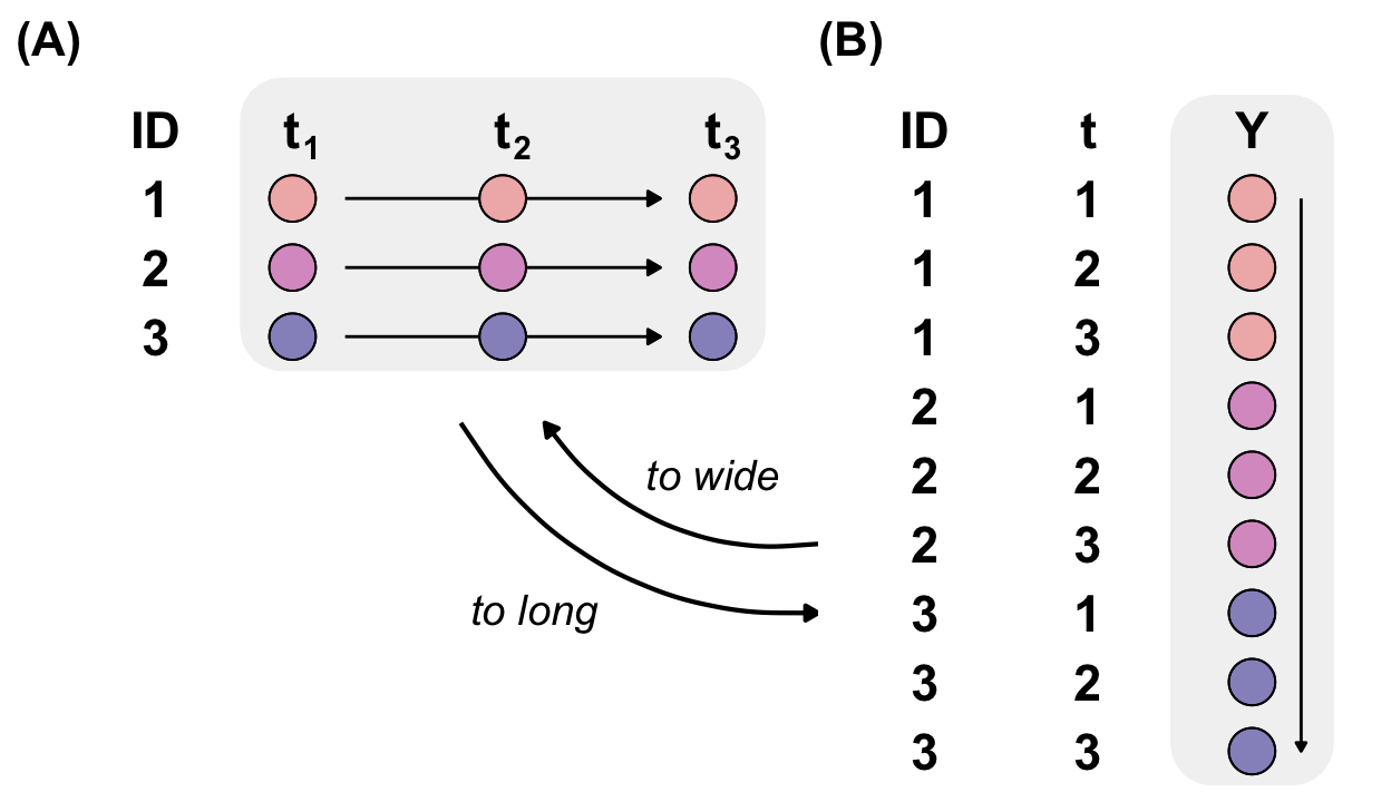
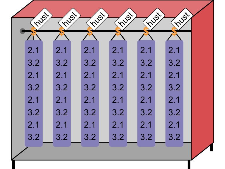
Two types of data storage in the wide and long format. It is important to remeber, that we need the long format for the visualitation and analysis in R. The wide format is also called unstacked data. We use this type of data, if we measure time series data or data which is changing in the same subject. In this applications, the format is very effiecent to store but difficult to analyse. The long format is also called stacked or narrow data. The long format is the standard format for the analysis of data. The measured variable Y is only contained in one column.
2.4.2 The elephant in the room is Excel
What problems are there with Excel?
- Reach and shareability. If we do something in Excel by point and click, nobody else can do it if they are not observing us.
- Scalability and efficiency. If we have one task, it will take some time. If we have the same task with different numbers, it will take twice as long. We cannot really automate any processes.
- Excel is error-prone. If we make a mistake, we will not really understand why things did not work. We can click again, but we have no protocol to follow. Others cannot understand what we have done.
- Excel is neither open nor free to use. We need a licence to use Excel and are unable to share any files with people who do not have access to Microsoft products.
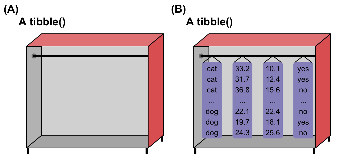
2.4.3 Tidy data
2.5 R packages used
Do we want here to simulate data?
2.6 Data
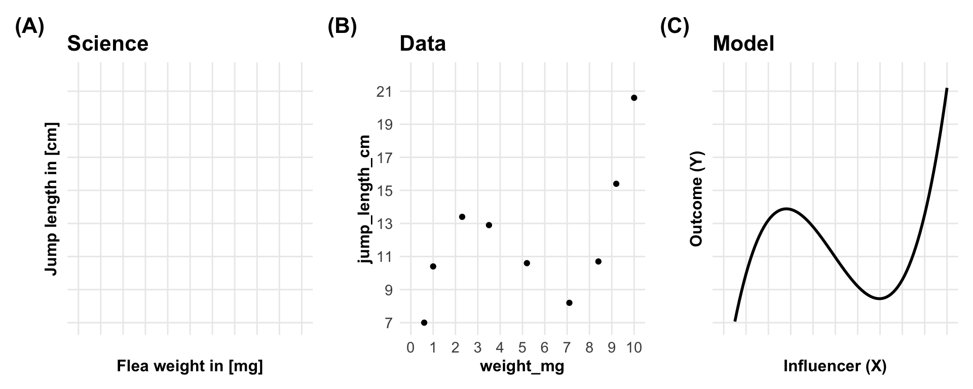
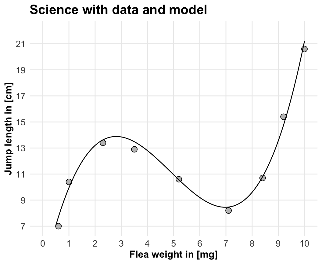
Is your data the fuel of discovery or the test of discovery?
R Code [show / hide]
jump_weight_tbl <- tibble(x = c(0.6, 1, 2.3, 3.5, 5.2, 7.1, 8.4, 9.2, 10),
                          y = 0.15*x^3 - 2.2*x^2 + 8.8*x + 3.2 + rnorm(9, 0, 0.5)) |>
  mutate_all(round, 1) |>
rename(weight_mg = x, jump_length_cm = y)| weight_mg | jump_length_cm |
|---|---|
| 0.6 | 8.5 |
| 1.0 | 9.6 |
| 2.3 | 13.7 |
| 3.5 | 13.2 |
| 5.2 | 11.0 |
| 7.1 | 8.3 |
| 8.4 | 10.9 |
| 9.2 | 14.3 |
| 10.0 | 21.1 |
\[ y = 0.15\cdot x^3 - 2.2\cdot x^2 + 8.8 \cdot x + 3.2 \tag{2.1}\]
2.7 Outro
What do we want to do in this book? We want to perform inductive reasoning based on data. Statistical modeling is inductive reasoning, so it is also based on data. Therefore, we will need data to perform statistical analyses in any possible combination. In other words, we live in a data-driven world.
In this book, we will follow an inductive approach. First, we make observations, then we try to find patterns in them. Therefore, our data is the fuel of discovery. Conversely, we can also use data to test a hypothesis. Both are valid and are used. Since this book is about statistics and data science, we cannot generate new theories. We are limited by the tools we have and the data available to us. This book may be read by those with a background in natural science. Then, you can use the statistical tools differently.
2.8 Alternatives
Further tutorials and R packages on XXX
2.9 Glossary
- term
-
what does it mean.
2.10 The meaning of “Models of Reality” in this chapter.
- itemize with max. 5-6 words
2.11 Summary
References
[1]
Boese A. Electrified Sheep. Pan Macmillan UK; 2011. https://books.google.de/books?id=8Cgb5MD88AoC
[2]
European Commission. Guidance on the Validity of Clinical Studies for Joint Clinical Assessment. Directorate-General for Health; Food Safety; 2024.
[3]
Toumi M, Falissard B, Jouini A, Aballéa S, Boyer L. Clinical trial validity guidance from the HTACG: Looking for chicken teeth. Journal of Market Access & Health Policy. 2025;13(2):15-15.
[4]
Dormann CF, Ellison AM. Statistics by Simulation: A Synthetic Data Approach. Princeton University Press; 2025.
[5]
Hassenstein MJ, Jung K. Ten simple rules for effective research data management. PLOS Computational Biology. 2025;21(12):e1013779.
[6]
Wilkinson MD, Dumontier M, Aalbersberg IjJ, Appleton G, Axton M, Baak A, et al. The FAIR guiding principles for scientific data management and stewardship. Scientific data. 2016;3(1):1-9.